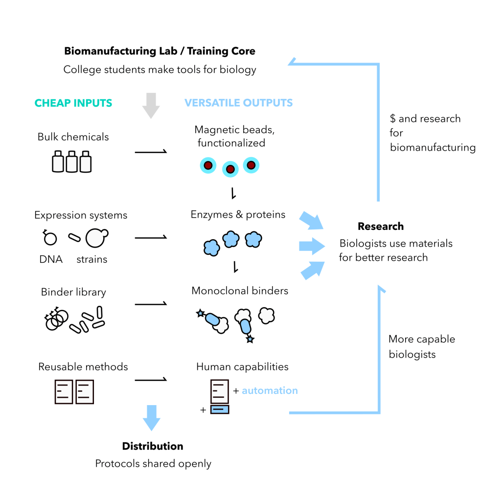
What if universities used undergraduates to make biological reagents? Training people in biomanufacturing, and using their outputs, could reduce research costs with plenty of other benefits.
Here’s a diagram of how I think this would work:
The problems a college biomanufacturing core touches are: (1) giving more students opportunities for meaningful hands-on experience, (2) training a workforce for the bioeconomy, (3) biology is expensive, (4) insane cuts to science funding by the U.S. government
It can be economical & bootstrappable, I think, to focus on: reusable paramagnetic beads for purification, proteins synthesized by microbes, and synthetic monoclonal antibodies. The outputs are versatile, yet the process is standardized, the inputs are cheap. You make most of what you need.
A lot of academic labs already make their own enzymes, but the cost-benefit doesn’t always make sense for 1 lab. That’s why New England Biolabs exists. Formalizing a program to service all labs adds benefits: more students trained, more reagents made, more network effects as labs cooperate.
For the perspective of an individual lab, these services may not save much money, but more money stays in the university for training and education instead of being paid out to third party companies and their investors.
And there are other important benefits: (A) These students will take their know-how with them to make an impact in new labs and companies. A lot of good research hasn’t happened because people didn’t have that kind of agency. (B) These cores may inspire new research – like new molecular tools, automation methods, and ways to have a global impact by sharing affordable production methods. (C) Colleges can specialize for the purposes of branding e.g. add a module for plant genome editing or industrial fermentation. They may even consider programs, similar to agricutlural extensions, that help small biotech operations get off the ground.
How to start?
If you run a lab course, change the last section to be making an enzyme to give to your department, then add.
If you’re hiring students for summer research, have their project be setting up this service for your university.
Someone could have an outsized impact across universities by establishing the key protocols that together are economical, creating collaborators, and making an open system for sharing protocols and materials. What’s the essential seed for another college to start?
I recommend reading this blog post if you are a microbiologist interested in (1) isolating more diverse organisms, (2) characterizing metagenomes in more detail, or (3) understanding why genomes are the way they are. This blog post will help you build on my preprint with Cultivarium, “Predicting microbial growth conditions from amino acid composition“, which provides a tool called GenomeSPOT. I recommend reading the preprint, especially to understand the limitations of the tool.
What’s Cultivarium? It’s a focused research organization from Schmidt Futures that’s producing tools and data to accelerate microbiology research. Check out resources for genetics (here and here and here) and stay tuned (cultivarium.org and @CultivariumFRO).
What’s the preprint? You want to know the conditions a microbe needs to grow. Previous research has provided models to predict optimum temperature for growth from amino acid composition and described correlations between optimum salinity and amino acid composition. We extend that work to provide models for not only temperature but also salinity, pH, and oxygen.
Why does that matter? We can now describe microorganisms in nature in terms of their physical and chemical niche. We can use this to learn find our if we’ve been doing anything wrong in cultivation. We can further explore why these and other conditions influence microbial growth through the cost of protein biosynthesis.
Understanding the models
A brief explanation of models
We wanted to predict a variable like optimum growth temperature, which we’ll call the “target.” We had available a variety of data measured from a genome, which we’ll call “features.” We took a model, like a linear regression, and “fit” it to the training data. What the means is that the model found the way to weights and combinations the features in order to optimally predict the target. Different models have different ways of weighing and combining features and different ways of “scoring” the best fit. As you can imagine, the features with the strongest weights are often those most correlated to the target variable.
The risk with modeling is that the model doesn’t apply to new examples. The weights and combinations that provide a good prediction of the target for one set of genomes may not work for another set of genomes. That’s may seem counterintuitive, but remember that spurious correlations happen all the time and are more likely the more variables (features) you measure and the fewer examples (genomes) you use. Therefore, when we were choosing which models to use, we compared them by how well they scored on genomes that were held out of model training (“cross-validation”). We also held a “test” set of genomes out that were not used in model training or selection in any way but reserved to check that the model was still predictive on new organisms
In microbiology, spurious correlations can result from the phylogenetic relationships, so we — as everyone should — took steps to account for these biases.
The oxygen / amino acid surprise and why it matters
The biggest finding is that amino acid composition is so influenced by oxygen, so it’s a good place to build an understanding.
Here’s how non-obvious this finding is: I tried to predict oxygen with amino acid composition because I thought it wouldn’t work, and I was worried at first when it did work. My expectation of amino acid composition was that extremes of temperature, pH, salinity could shift some amino acids but that overall composition is influenced by (A) the influence of GC content on codon usage, (B) phylogenetic history, and (C) not much else. Was this model just biased by GC content and phylogeny?
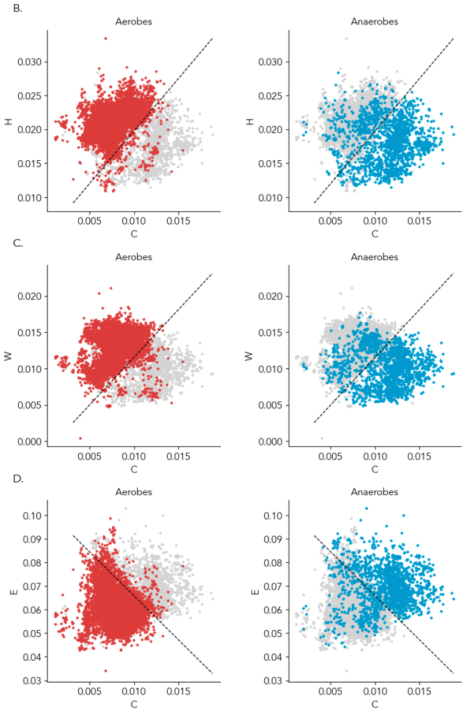
In the preprint, we show amino acids predict oxygen in a GC content and phylogeny independent way. For those skeptical of modeling, the most compelling data is that just two amino acids can provide a ~90% accurate classification of a microbe as aerobic or anaerobic, and you can see the clustering yourself in the below scatter plot (Supplementary Figure 4). Specifically, the average frequency of cysteine with histidine, tryptophan, or glutamate (glutamine is a runner up) in the genome is enough to know if a microbe can live in the presence of oxygen or cannot. In the plot below, a line from a logistic regression uses the amino acid frequencies on the x- and y- axes to classify microbes as aerobes or anaerobes (highlighted in left and right plots). ~95% of aerobes and ~85% of anaerobes fall on either side of the line. That isn’t machine learning magic; it’s real, tangible biology. And interpretable: we can try to understand why some anaerobes are in the aerobe “region”.
Supplementary Figure 4B-D. Each dot is a genome. x-axis is the genome’s cysteine frequency and y-axis is the frequency of another amino acid highly correlated with oxygen. The data in the left and the right plots are the same, but in the left plot aerobes (obligate and facultative) are colored and in the foreground, and in the right plot anaerobes (presumed obligate) are colored and in the foreground
We haven’t had good ways to classifying a microbe as an aerobe or obligate anaerobe. Doing it from genes is not as straightforward as you’d think. Even obligate anaerobes have oxygen tolerance genes like catalase or peroxide and genes for using oxygen as a respiratory electron acceptor, so a manual determination is tricky. Gene-based models to provide automated prediction of oxygen tolerance appear good (especially Davin et. al 2023), but there’s always a nagging worry about how well they work for new groups of life or for incomplete genomes. I expect the new model to be very helpful because it’s grounded in biological first principles.
Specifically, we hypothesize oxygen influences amino acid content for bioenergetic reasons:
Sulfur assimilation take a lot more energy when you have to reduce sulfate (oxic habitats) than when there’s a lot of reduced sulfide around (anoxic habitats). Also, oxidation of cysteine to cystine causes some important problems for microorganisms. Solution: to become an aerobe use less cysteine. (Full credit to Paul Carini for this insight).
Respiring oxygen provides a lot of energy, making energy-intensive amino acids relatively less costly. Solution: if you’ve become an aerobe, it’s OK to use more histidine and tryptophan over less costly similar amino acids.
A critical decision was to lump everything but obligate and unspecified “anaerobes” into aerobes: aerotolerant anerobes, microaerophiles, facultative aerobes, facultative anaerobes, simply “aerobes,” and obligate aerobes. Researchers have been close to finding the patterns we described for decades (Naya et. al 2002, Vieira-Silva & Rocha 2008) and even recently (Davin et. al 2023, Flamholz et. al 2024), but how to classify facultative anaerobes complicated their analyses. We decided to lump them together because compared to obligate anaerobes both aerobes and facultative anaerobes have similar numbers of oxygen-utilizing enzymes (Jablonska & Tawfik 2019). We found that in terms of amino acid composition, too, facultative anaerobes are essentially aerobes.
I recommend the following decision tree to classify microorganisms by oxygen use:
GenomeSPOT predicts not oxygen tolerant: Obligate anaerobe
GenomeSPOT predicts oxygen tolerant:
Has genes to respire oxygen: Aerobe
Has genes to respire other electron acceptors or to perform fermentation: Facultative anaerobe / facultative aerobe
No other energy sources: Obligate aerobe (in practice hard hard to be confident)
Does not have genes to respire oxygen: Aerotolerant anaerobe
Four suggestions for better isolations inspired by this work
70% of microbial species, classes, etc. are not isolated (source: GTDB). With our tool we could show that are enriched in anaerobic and thermophilic microorganisms. Among the metagenomes researchers have chosen to sample, those organisms are ~50% and ~20% of species and x- and x-fold underrepresented in culture collections. (Note that because most microbial biomass in the subsurface, it’s likely that current sampling underestimates the diversity of anaerobes and thermophiles).
Use anoxic conditions and higher temperatures to isolate more novel organisms
Anoxic conditions are obvious, but why is 37C not good enough to culture moderate thermophiles? After all, they should grow at that temperature.
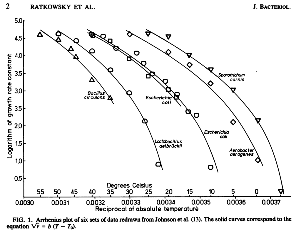
Due to the Arrhenius relationship between temperature and biochemical reactions, at 10C below optimum temperature microbes grow at half the rate . When we already have an isolate, we may be OK with growth conditions that are simply permissive. But during isolation, when microorganisms are competing with one another, this halved growth rate would lead to out-competition by colonies with optimum temperatures equaling the incubation temperature. For example, in the below plot from Ratkowski et. al 1982, at 35C Lactobacillus delbruckii (optimum ~47C) grows at a 1/e the rate (1 natural log less) of Escherichia coli (optimum ~37C), which adds up over the many generations required to produce a colony. Beyond a 10C drop in temperature, the drop in growth rate exceeds the Arrhenius relationship.
Is it the temperature making you sweat or is that 45-60C is a lot harder to work with than 25-37C because of issues like agar gelling and water evaporation? Weigh the costs with the benefits of increased diversity and potential relevance for biotechnology. Getting set up for higher temperatures and sampling slightly higher temperature environments (near subsurface, sun-baked soils and sediments, warm climates, etc.) could be worth the cost.
Worry about the oxidation state of media components provided to anaerobes
Seeing the influence of oxygen content on amino acid composition, especially cysteine, makes me imagine that the media we provide anaerobes could be toxic to many anaerobic lineages. Uncultivated anaerobes tend to have higher cysteine content than cultivated anaerobes (data not shown in preprint), hinting that this is indeed the case.
I think I used the same stock of cysteine as a reductant for my entire PhD, and I removed oxygen from medium components like yeast extract by sparging but never chemically reduced them. What if cystine (oxidized cysteine) in those media components inhibited most of the strains in samples before I could isolate them? I usually provided sulfate as a source of sulfur. What if many species require sulfide or cysteine as a source of sulfur instead? What if – here’s what may be new ideas – many anaerobes can’t be isolated because in order to grow well they require a partner organism to detoxify cystine to cysteine or reduce sulfate to sulfide?
Provide different combinations of growth conditions based on metagenomics
Using this tool with metagenomics, you can describe the growth conditions of all microorganisms in a community. Therefore, you can estimate roughly what portion of species will grow at a given pH, salinity, temperature, and oxygen condition. In many cases you will find that using 1 or 2 media is only able to isolate a small minority of the diversity of a community. Try a few more media at different conditions. If you don’t have a metagenome for you sample, refer to the data by habitat from the JGI Genomic Catalogue of Earth’s Microbiomes provided as a supplement.
Don’t use this tool as the sole motivation for targeted isolation
“A tool to provide growth conditions for metagenome-assembled genomes will help me target a specific organism for isolation!” – someone leaping before they look. Targeted isolation of a single microbe is very laborious and high risk. Many microorganisms will not grow because of other reasons than the right growth conditions haven’t been tried. You can use the tool for targeted isolation, and anyone already doing targeted isolation should use the tool, but you should probably just use this tool to maximize the diversity you can capture from a given habitat, as discussed above.
Using this tool for metagenomics
Metagenomics has provided astounding insights into microbial biology, especially phylogeny, metabolic diversity, and biological interactions of uncultured microorganisms. Working in soil metagenomics at Trace Genomics made me appreciate that the physical and temporal variability of microbial communities, which is at its peak in soil. In many microbial environments, what looks like a homogenous environment to us is very heterogeneous on the micro-scale. GenomeSPOT is therefore useful in two ways:
This tool allows us to describe individual microorganisms in terms of physical and chemical niche. What can learn about ecology now that can estimate these traits?
This tool allows us to represent communities in terms of distributions of physical and chemical niches.Kurokawa et. al 2023 showed how an essentially identical prediction of optimum growth temperature can serve as a “thermometer” for the temperature experienced in microbial communities. Now you can also try** that for salinity, pH, and oxygen. (** we didn’t test the average predicted condition for a community to real measurements, so this remains to be proven). We really didn’t explore this too much, leaving the fun analyses to the reader.
Thinking at the microscale may help to explain why we see elevated temperature be more common. Sunlit surfaces can temporarily be much hotter than their surroundings. Perhaps there are lots of hidden thermophiles that grow only when the sun is shining. One indication of this is the high average optimum temperature for microorganisms from the surface of macroalgae (Fig 4A).
Bread crumbs for genomics
Explaining DNA and amino acid composition of genomes
Other factors that influence genome composition include nutrient limitation affecting amino acid usage (Grzymski & Dussaq 2012), and mutations in DNA due to environmental factors (Ruis et. al 2023, Aslam et. al 2019, Weissman et. al 2019). The finding that growth conditions, especially oxygen, influence amino acid composition makes it tantalizing to try to create a causal model of how a microorganism’s niche influences its genome.
A helpful starting point could be comparing whether metabolism and/or habitat influences where an organism resides in “amino acid space.” For example, I noticed in plots of oxygen-influenced amino acids like cysteine vs. histidine, dissimilatory sulfate-reducing bacteria clustered together (with high Cys content) and anoxygenic phototrophs clustered together (with aerobe-like Cys content). Then there are interesting exceptions, like the fact that cultured Campylobacterota, which are mostly microaerophilic, tended to look like anaerobes in cysteine content.
Evolutionary transitions
One exercise left to the reader was performing the in depth analysis of the phylogenetic distribution of growth conditions. How many times have different conditions evolved? How phylogenetically conserved are they? Are conditions even distributed across Archaea and Bacteria or do certain groups tend to have different conditions than others? An example of this work using extreme halophiles in Archaea just came out this week. There are lots of interesting questions left for you to tackle.
Finding genes related to physicochemical conditions
We chose to not build a gene-based model because we wanted to build something that would be accurate for new organisms. Before trying to predict a traits with genes, you should ask yourself: of all the genes in all microbes that influence this trait, what % are found in organisms in my training dataset? For a single deeply conserved pathway like denitrification, that representation might be very high, perhaps >99%. For a complex trait with many genes involved like living in a particular temperature/pH/salinity, we suspected it’s unlikely cultivated microorganisms could represent uncultivated microorganisms.
Ironically, the sequenced-based models we’ve provided might change that equation. Now you do have data on growth conditions for diverse microorganisms on which to build models. I recommend people try this, with a couple important suggestions:
Select a subset of genes to be features. Models overfit when there are too many features relative to the training data. You should only feed in genes to a model that you have linked to conditions. This feature selection can be part of a model training pipeline, or it can be a separate investigatory process.
When selecting genes, use held out taxonomic clades to test the selection. This is the most likely place where you will mess up and introduce data leakage: you find the genes most correlated to optimum pH across all genomes, then you use those genes to build and test a model with proper cross-validation and test sets. Where did you go wrong? When you selected correlated genes, you use all genomes, including those later in the test set, which means that your model had access to test set information. To truly know if your gene-based model is robust to phylogeny, you need to holdout test data from feature selection as well as later modeling steps. Ideally, feature selection is part of a model training pipeline.
Account for missing or multicopy genes in metagenome-assembled genomes. I recommend emulating the modeling work described in the Davin et. al 2023, where they used a gradient boosted regression model trained on genomes with random gain or loss of genes. If you see in training you can’t accurately predict growth conditions on genomes with missing or multicopy genes, your model won’t work in practice on MAGs.
Your work could identify the genes that correlate with life at different temperatures, pH, and salinities, which could be helpful for biotechnology.
Wrap-up
The Cultivarium team hopes this tool provides a lot of value to researchers. I hope this blog post has provided you with a new interest in growth conditions and genomics and some ideas of what to research next. Feel free to reach out with any questions.
Disclaimer: This blog post is a primer intended for scientists and policymakers with an interest in limiting methane emissions from cattle. My qualifications are that I am a microbiologist with expertise in microbial metabolism. I have studied microbial metabolisms, authored a review on the biogeochemistry of chlorine, and obtained my Ph.D. in a laboratory studying chemical inhibitors of metabolism. I am not an authority on business/investments/law/animal husbandry and my analysis of any companies mentioned here should not the basis of any business/investment/legal/animal husbandry decisions.
Humanity has a methane-from-cattle problem. Our herd of 1 billion cattle is over 8 times the weight of all wild animals. In the United States, our herd size hovers about 100 million cattle. Cattle, like other ruminants including sheep, have an extra stomach full of microorganisms, called a rumen. The microorganisms in the rumen help digest otherwise indigestible plant matter, allowing the animal to obtain more nutrients from its food. Unfortunately, a byproduct of this fermentation is methane: a potent greenhouse gas, produced by specific microorganisms in the rumen, burped out by the cattle. Scientists call this “enteric methane,” referring to digestion. The feed, waste, and burping of the vast mass of ruminant livestock accounts for about 14% of global greenhouse gas emissions, with enteric methane accounting for about 4% of global emissions. Unlike a sector like energy production, where technology exists to reduce greenhouse gas emissions, enteric methane emissions has been a point of pessimism: in my view, people will always eat beef, and it is not like you can swap out a rumen with a new stomach part that doesn’t make methane. Reducing emissions from feed and waste – important parts of livestock’s life cycle emissions – is indeed feasible, and in feedlots, where cattle spend a portion of their lives, enteric methane might be physically captured. Yet absent a cheap, portable way to stop the microorganisms that make methane, cattle will continue to emit massive amounts of methane for the foreseeable future.
But nowwe do have technology for enteric methane mitigation. As headlines like “Pellet That Stops Cows From Burping Climate-Warming Methane” (Bloomberg, November 29, 2022) allude to, these are drugs that act as antibiotics against the microorganisms that produce methane. The most effective technology reduces cattle methane emissions by 50-90%, with room for improvement. There’s a catch: the technology is the use of halomethanes like bromoform to inhibit methane-producing microorganisms. Halomethanes degrade the ozone layer.
Here I lend a primer, with my views, on the complications of using halomethanes to stop methane emissions from the rumen. These compounds appear to be an effective, cheap, and scalable solution that businesses can develop and profit from. To those of us hoping for another winning solution against climate change, these compounds cannot go to market fast enough, and commercial hurdles for these companies ought to be cleared. However, halomethanes come with concerns, the most serious of which, the potential for degrading the ozone layer, has major repercussions that scientists ought to address, perhaps before the technology is deployed. Finally, as a microbiologist in this scientific area, I feel like we have failed to provide adequate alternatives to address methane mitigation, and I end with a call to action for microbiologists to work on this important problem.
Halomethanes as a way to stop methane production
The microorganisms that produce methane are called methanogens. Like many microorganisms, they have a metabolism that looks nothing like our metabolism. We turn carbon (food) into energy by respiring oxygen, releasing water and carbon dioxide as byproducts. Methanogens obtain energy by converting carbon dioxide, hydrogen, and other compounds into methane. There are different types of methanogens, but all methanogens are single-celled microorganisms in the domain of life called Archaea, which diverged from the domain Bacteria early in Earth’s history. Life as a methanogen is hard: not only are they are sensitive to oxygen, but their metabolism provides very little energy. In order to survive, they need to churn out large amounts of methane. Microbial habitats with little oxygen and lots of organic matter, like the cattle rumen, lead to a lot of methane, perhaps as much as 10% of the carbon fed to the cattle.
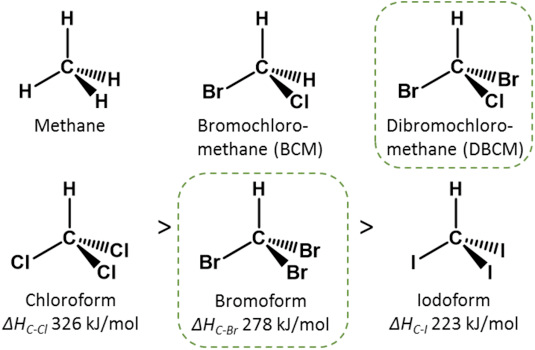
Halomethanes affect methanogens because they look like methane. A molecule of methane is a carbon atom surrounded by 4 hydrogen atoms. Unlike methane, halomethanes have one or more hydrogen atoms replaced by an atom of a halogen element such as chlorine or bromine. As early as 1968, microbiologists recognized that the chemical similarity of methane and halomethanes meant that halomethanes would interfere with the enzymes responsible for producing methane, like how a wrench fitting between gears can stop their turning (Wood et. al 1968). Halomethanes interfere with the cellular machinery that makes methane.
Caption: Structures some halomethane molecules compared to methane. Source: Glasson et. al (2022). Benefits and risks of including the bromoform containing seaweed Asparagopsis in feed for the reduction of methane production from ruminants. Algal Research
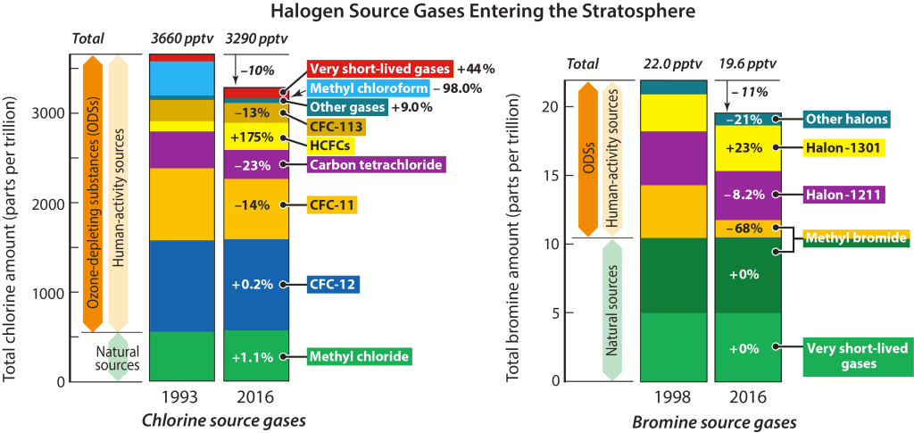
The primary issue with halomethanes is that they are gases that can carry halogen atoms aloft. As NOAA explains, above the lower atmosphere, in the stratosphere, is a layer of ozone that protects us by limiting how much ultraviolet radiation reaches Earth’s surface. Halogen-containing gases that persist long enough in the atmosphere can reach the stratosphere. Once in the stratosphere, gases containing halogens can be broken apart, releasing atoms of chlorine or bromine that catalyze the destruction of ozone. With less ozone to absorb ultraviolet light, more UV penetrates the stratosphere and reaches us. The dangers of higher UV exposure led all countries in 1987 to agree to Montreal Protocol phasing out the production of chemicals that destroy the ozone layer, including many halomethanes and all chlorofluorocarbons. (The Montreal Protocol was updated in 2016 to phase out certain halomethanes that are potent greenhouse gases but not ozone-depleting). The Montreal Protocol does not regulate very-short lived gases though recent research indicates these compounds do pose a risk.
A secondary issue with halomethanes, that I do not discuss beyond here, is that they not inert pharmaceuticals that only bind a specific drug target. Halomethanes can act as solvents or as donors of halogen elements to other molecules, resulting in toxicity. For example, chloroform (CHCl3) at high concentrations can affect liver function and cause mutations leading to cancer (US EPA factsheet). Toxicology is a consideration for any drug, and dose determines determines the effect. So far, trials have demonstrated inhibition of methane inhibition at apparently safe doses. Perhaps there may always be concerns about health risks, even in animals with a short lifetime, among livestock growers (e.g. “Hold off — for now — on feeding seaweed to cows to reduce methane.”) Yet this could be true for any drug given to livestock. The other inhibitor of enteric methane in use, 3-nitropropanol, is also toxic at high enough doses and could have optics issues.
A slow path to seaweed as a source of halomethanes
The Montreal Protocol also eliminated the most obvious solution to cattle emissions. Initial research in the 1990s and 2000s show promising results for bromochloromethane (CH2ClBr, or “BCM”), commonly used by microbiologists to specifically inhibit methanogens, to stop methane production in the rumen. However, the Montreal Protocol scheduled a stop to bromochloromethane production in 2002. A paper published in 2009 reads as a “swan song” for bromochloromethane:
The experiments reported here were completed in 2004 before the Australian Government prohibited the manufacture and use of [bromochloromethane]. It is unlikely that the [bromochloromethane] formulation will be available for commercial use to mitigate livestock methane emissions in Australia. Nevertheless, the study has demonstrated that methane emissions were substantially reduced over a 90-day feedlot finishing period. This indicates that alternative antimethanogens with a similar mechanism of action may have practical commercial relevance.
Tomkins, N. W., Colegate, S. M., & Hunter, R. A. (2009). A bromochloromethane formulation reduces enteric methanogenesis in cattle fed grain-based diets. Animal Production Science, 49(12), 1053-1058.
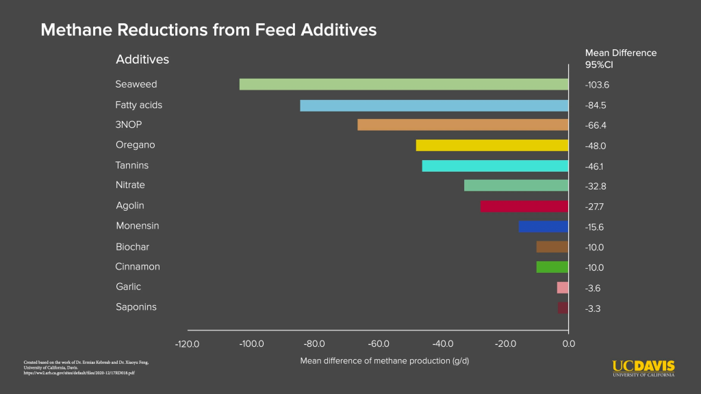
With few alternatives identified by microbiologists, animal researchers began to test diverse feedstocks or feed ratios hoping for something to work. The scientific term for this is “throwing things at the wall and seeing what sticks” (humor). Compounds ranged from known inhibitors of methanogen production like fatty acids to various feed additives like cinnamon, garlic, seaweed, and oregano. Where this research stood in 2014 is summarized in this report sponsored by the UN Food Agriculture Organization. One of the successes based on microbiology research, 3-nitropropanol, shows reductions of methane of about 30% and is commercialized by DSM under product name Bovaer. Yet the substance that showed the most reductions in methane was a specific dried red macroalgae Asparagopsis taxiformis, or its cold-water cousin Asaragopsis armata. (Marine macroalgae = seaweed). As scientists like Ermias Kebreab at U.C. Davis have shown to widespread media attention, Asparagopsis can reduce methane emissions over 80%.
You might expect the classic story: after testing substances for bioactivity, scientists find a promising substance and isolate and synthesize the active ingredient. However, the active ingredients in Asaragopsis are… halomethanes. Specifically, Asaragopsis has high amounts of bromoform (CHBr3) and dibromochloromethane (CHClBr2). A number of publications stated that these compounds were prohibited under the Montreal Protocol. For example, here is the key paper establishing the active ingredients in Asparagopsis:
Despite the demonstrated efficacy at low concentrations, the use of artificially formulated HMAs [(halogenated methane analogues)] in livestock production systems is prohibited because of their ozone depleting effect. Naturally derived sources of HMAs may provide a practical alternative method for delivery into the rumen. The red macroalga (or seaweed) Asparagopsis taxiformis produces high concentrations of [bromoform] as a secondary metabolite, which accumulates within vacuoles of gland cells.
Machado, L., Magnusson, M., Paul, N. A., Kinley, R., de Nys, R., & Tomkins, N. (2016). Identification of bioactives from the red seaweed Asparagopsis taxiformis that promote antimethanogenic activity in vitro. Journal of Applied Phycology, 28, 3117-3126.
Perhaps out of concern these compounds were prohibited, a number of startups, like Symbrosia and Blue Ocean Barns, began selling Asaragopsis seaweed instead of synthetic bromoform/dibromochloromethane. These companies have had impressive breakthroughs in cultivating algae through aquaculture, instead of harvesting wild seaweed, and in breeding seaweed with improved properties. Blue Ocean Barns is currently testing their product with two upscale California dairies, Straus and Clover. Both companies have done great work that deserves praise. Yet, while cheaper than harvested seaweed, aquaculture-grown seaweed is still expensive. Symbrosia estimated a cost of $0.80-1.50/day per cattle for their product, perhaps cheaper later, and presumably Blue Ocean Barns would be similar. The product from Blue Oceans Barns is paid for by carbon offsets market to prevent emissions, a relatively great use of offsets that we might expect adopted by other seaweed producers. However, at that cost, can offsets scale to continuous use in hundreds of million of cattle?
This begs the question: are bromoform/dibromochloromethane really prohibited by the Montreal Protocol?
Caption: Promotional material by Blue Ocean Barns
Caption: Reporting by Verge on Symbrosia
The promise of synthetic halomethanes
Ozone depletion is caused by human-related emissions of ODSs [ozone-depleting substrances] and the subsequent release of reactive halogen gases, especially chlorine and bromine, in the stratosphere . . . The substances controlled under the Montreal Protocol are . . . long-lived (e.g., CFC-12 has a lifetime greater than 100 years) and are also powerful greenhouse gases (GHGs) . . . In addition to the longer-lived ODSs, there is a broad class of chlorine- and bromine-containing substances known as very short-lived substances (VSLSs) that are not controlled under the Montreal Protocol and have lifetimes shorter than about 6 months. For example, bromoform (CHBr3) has a lifetime of 24 days, while chloroform (CHCl3) has a lifetime of 149 days. These substances are generally destroyed in the lower atmosphere in chemical reactions. In general, only small fractions of VSLS emissions reach the stratosphere where they contribute to chlorine and bromine levels and lead to increased ozone depletion
If the only point of using seaweed was to circumvent the Montreal Protocol, then using seaweed has no point. The UN World Meteorological Organization, the authority on this matter, states that as very-short lived gases, the active ingredients in Asparagopsis are not regulated by the Montreal Protocol. Perhaps they should be, but they are not. Even if they were regulated, these compounds are chemically no different synthesized by algae or synthesized in a factory. If using seaweed to synthesize prohibited halomethanes was a loophole in the Montreal Protocol, we might want to close it.
Halomethanes are very cheap to synthesize using existing chemistry, like the haloform reaction, and halogens extracted from seawater and brines with existing technology (e.g. Octel Bromine Works). Huge amounts of bromine are extracted from brines (and, previously, seawater) from the United States and Israel for synthesizing molecules containing bromine. Bromoform can be purchased in bulk at $0.01 per g (lowest observed quote on vendor websites). An effective dose of Asaragopsis delivers 0.39 g bromoform per day to cattle, meaning the equivalent amount of bromoform would be <$0.01/day per cattle compared to the cost of Asparagopsis at roughly $0.80/day per cattle. Added costs will come from delivering the compound to livestock, which as a gas is trickier than adding powdered seaweed to feed. But gases can be in encapsulated feed, like carbon dioxide in pop-rocks candy, or provided in a slow-release “bolus” object shoved into the rumen, which allows grazing animals outside of feedlots to be dosed.
Caption: Industrial-scale bromine extraction from seawater at Octel Bromine Works
Synthetic halomethanes are a low-cost solution that can scale as a business. In some instances, methane inhibition has led to faster cattle growth because less carbon is lost to the atmosphere. If the product can be cheap enough to pay for their benefits to cattle growth, cattle growers will pay for it. If not, it’s still a solution that stretches offset funding further, and public policy can aid adoption. Either way, the lower cost advantage is an obvious business opportunity, with an addressable market of hundreds of million of cattle. A new company, Rumin8, uses a feed containing synthetic bromoform, recently received investment from Breakthrough Energy Ventures, and is “on a mission to decarbonise 100 million cattle by 2030.” A new company’s interest is to secure an advantage over likely competitors by building barriers to entry (patents, client relationships, lower unit costs, etc.). Our interest, as a public that wants to limit climate change, is to have several companies providing inhibitors of methane so that prices remain low and more of the market is reached. Based on existing patents and the potential for different delivery options and co-formulations, my opinion is that there is room for a smart company to enter the market successfully.
An argument for Asaragopsis over synthetic halomethanes is that the seaweed currently shows higher efficacy in reducing methane than pure bromoform, perhaps because of different rate of release or the presence of other halomethanes buttressing bromoform. There’s no reason why synthetic halomethanes formulations cannot be optimized to have the same or even greater efficacy than seaweed. With synthetic product instead of an algal product, rate of release can be more easily controlled. Plus, companies could choose from a wide list of very-short lived halomethanes, most of which should be expected to inhibit methanogens, to maximize efficacy while minimizing downsides (cost, health risks, ozone depletion potential, global warming potential, etc.). Companies would be advised, at a minimum, to consider using both bromoform and dibromochloromethane to mimic Asparagopsis. (Very-short lived halomethane gases not regulated by the Montreal Protocol include at least the following: dichloromethane (CH2Cl2), chloroform (trichloromethane, CHCl3), tetrachloroethene (CCl2CCl2), trichloroethene (C2HCl3) and 1,2-dichloroethane (CH2ClCH2Cl), bromoform (CHBr3), dibromomethane (CH2Br2), bromochloromethane (CH2BrCl), dibromochloromethane (CHBr2Cl), and bromodichloromethane (CHBrCl2), methyl iodide (CH3I), iodochloromethane (CH2ICl), diiodobromomethane (CH2IBr), diiodomethane (CH2I2) and ethyl iodide (C2H5I)).
Seaweed would have taken a long time to scale up production, so perhaps scientists and policymakers expected more time to think. With synthetic halomethanes, the rate limiting step could be simply how quickly the products will be approved and adopted by the market. How many years would it take for large animal feed manufacturer like Cargill from buying a Rumin8-like company for its intellectual property and adding encapsulated bromoform to its products? 2 years? 5 years? Cutting methane emissions has an immediate, important impact on warming. The urgency of the climate crisis means that there will be enormous pressure to scale this technology whether scientists have properly evaluated the risks beforehand or not. Companies, investors, and some growers are certainly are not waiting. It’s time to evaluate synthetic methanes before their widespread use.
The risk of synthetic halomethanes
Reducing methane emissions from enteric fermentation by 50%, e.g. a market penetration of 50% of the global cattle herd of 1 billion at 100% methane mitigation, at 0.39 g bromoform per day requires the synthesis of at least 70 Gg of bromoform per year. Is it worth the risk posed by using so much of an ozone-depleting substance?
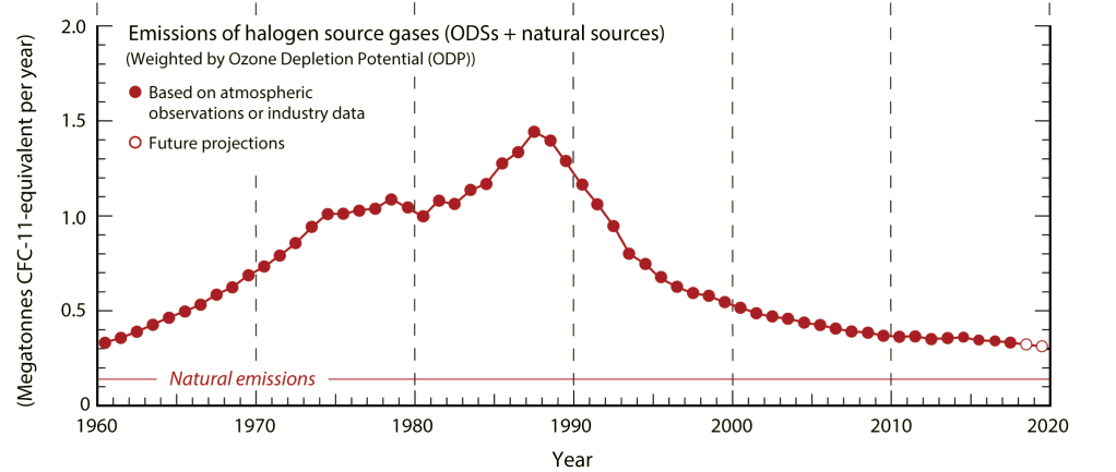
Very-short lived gases still contribute to stratospheric ozone depletion. Small amounts do live long enough the stratosphere through mixing, their breakdown products can be longer-living halomethanes like methyl bromide. A more important reason is that atmospheric mixing caused by monsoons gives gases a lift into the stratosphere. In the stratosphere, bromoform is particularly concerning because it carries three bromine atoms, and bromine is a more effective catalyst of ozone degradation than chlorine. The ozone depletion potential of emitted bromoform is estimated to be 1-5 times that of the same mass of CFC-11 (CFCl3), which is regulated by the Montreal Protocol. Methyl bromide has an ozone depletion potential of 0.57. (Ozone depletion potentials and global warming potentials of halomethanes are defined in Appendix Table A-1 of the Scientific Assessment of Ozone Depletion: 2018). It’s possible bromoform was not regulated simply because it was not synthesized in large quantities. The production of 70 Gg of bromoform per year, estimated above, means the potential emission of 0.07-0.35 Mt/year in CFC-11 equivalents (1 Mt = 1 billion kilograms). That is a very large amount considering annual emissions of ozone depleting gases are currently about 0.3 Mt/year, or double natural emissions. However, if we instead compare to the estimated natural emissions of bromoform at 120-820 Gg/year, synthetic production looks less impactful. (Hence why atmospheric scientists should be performing these analyses).
A key question is: How much of potential emissions will be realized? Halomethanes in the rumen are degraded by methanogens into halide ions like chloride and bromide. No longer in gas form, the risk posed by the halogen atoms has been eliminated for the moment. Companies have touted the degradation of bromoform and other halomethanes as a reason to be reassured about their use. Unfortunately, the science has some holes. We need to know more about the life cycle of halomethanes:
How much halomethane gas is released during production and distribution? Companies have some incentive to reduce loss of active ingredient from the product during distribution, as it reduces the quality of the product. However, as we learned with methane extraction from shale (“fracking”), without regulation, companies have no reason to prevent losses during production and manufacturing.
How much halomethane gas is lost from the livestock? Methane emissions from the rumen are measured but halomethane emissions are not. Intermediates of halomethane degradation must be measured. Methanogens removed halogen atoms one at a time: for bromoform, from three bromine atoms (bromoform) to two (dibromomethane) to one (methyl bromide) to zero (methane). Because molecules with more halogen atoms are more reactive, they will be degraded first while the intermediate products of the pathway accumulate. This has been shown for chloroform (Krone et. al 1989) and the same should be expected for bromoform and other halomethanes. Also of concern is how often bromoform is not degraded because no methanogens are left to degrade them. Scientists should better quantify how much halomethane is lost in eructed gases.
How much halomethane gas is made from livestock waste? In the ideal scenario that all halomethane molecules are converted to halides (e.g. bromide), the salts are excreted from the cow in urine and feces and end up in soil. The story does not end there. Halides are active in soils and can react with organic matter or be taken up by organisms. Bromide is particularly reactive and far less naturally abundant than chlorine. Most importantly, plants can convert bromide to methyl bromide, an ozone-depleting gas. The bromide in soils near the coast, where tides and winds lay sea salt, is one of the natural sources of methyl bromide emissions. In one study, plants immediately take up 95% of bromide added to soil and began to convert some to methyl bromide (Gan et. al 1998). If all bromide in soil ultimately makes it into the atmosphere, perhaps over many years, the use of bromoform in cattle will lead to methyl bromide emissions from soil. Understanding how much and how quickly this occurs is now a critical question.
How much will halomethane dose need to be increased? Dose might need to be increased for two reasons. First, as with other antibiotics, methanogens might evolve greater tolerance to halomethanes. Second, halomethanes might be degraded more quickly. Because some microorganisms benefit by breaking down halomethanes, these microorganisms might proliferate in rumens once halomethanes are more widely applied.
What is the strength of the ozone-depleting effect and the greenhouse gas effect for a halomethane gas? Choice of which halomethane matters. Gases vary in their ability to contribute to ozone depletion and global warming potential. Halomethanes other than bromoform will have different risk. Bromoform has a negligible global warming potential. Values for dibromochloromethane have not been determined, but bromochloromethane has a global warming potential 17 times that of carbon dioxide and about a fifth that of methane. There is also a geographic dimension to this question: extra precaution should be given to using ozone-depleting substrances in regions with higher risk of transport to the stratosphere, like southeast Asia.
In reality, because of the degradation of bromoform in the rumen, emissions of bromoform will likely be a very small fraction of the potential 0.07-0.35 Mt/year in CFC-11 equivalents. Until the above questions are answered, it would be precautionary to assume that a majority of bromine in bromoform delivered to cattle will ultimately be emitted. It’s also precautionary to limit global warming. Scientists should act now to (1) constrain the above questions to better understand emissions, (2) compare the benefits of enteric methane mitigation to the cost of ozone depletion, and (3) decide acceptable emission thresholds for enteric methane mitigation.
A useful role for public action
Let’s assume that there is some drug for enteric methane inhibition that we want governments to support, not prohibit. How should we do that? I am not an expert in advocacy or policy, but I want to raise the point that the infrastructure is not in place to mobilize this solution.
Compounds that inhibit methanogen production in livestock should have the opportunity to be given emergency regulatory approval. The emergency is the climate crisis. In the United States, at least, regulatory approval by the FDA is too onerous. Livestock growers must be confident that products are safe for use, but the process is too slow for the climate crisis we face. As of 2023, the product Bovaer, which leads to roughly 30% decline in methane emissions, is 6 years into the FDA process for approval as a drug for livestock, but it passed safety and compliance elsewhere and is in use in Europe and countries like Brazil. To avoid the same fate, Rumin8 and the producers of Asparagopsis seem to be trying very hard to be seen as “feed additives” instead of “drugs.” The FDA needs to continue to be lobbied to make the needed process changes, also requested by some in Congress, to expedite bringing drugs for enteric methane inhibition to market. This should have been done years to ago to create incentives for companies to develop solutions.
A more important barrier to adoption is that livestock growers currently have little incentive to use products that inhibit enteric methane production. The economic prerogative is for growers to sell tasty meat and milk, not to reduce methane emissions. Many growers will be averse the notion that their livestock are causing environmental harm. Enteric methane inhibitors could provide a growth advantage, which would lead slowly to adoption. But let’s assume they provide no benefit or an ambiguous benefit. Why take on an extra cost, not borne by your competitors, with no benefit?
A subset of customers who are environmentally conscious will pay a premium for products certified to produce lower methane emissions. I imagine many consumers would pay a hefty premium for certified “Low Methane” / “Minimal Methane” beef, milk, and cheese. The ability to obtain a premium from customers will create an economic incentive for many growers, though not all growers, to use a cost-effective methane inhibitor. Currently, there is no certifying organization. Should there be one, it ought to have a mission to provide an economic benefit to growers with truly low methane methods. An environmental organization with trust among growers should step into the void before organizations with other goals step in. For example, the American Feed Industry Association (AFIA) has been an advocate of this technology but make specious claims like “with just a 20-30 percent reduction in methane emissions, the entire livestock industry can be climate neutral in the next two decades.” We need a certifying organization to require close >90% reduction in enteric methane emissions, ideally plus emissions reduction through manure management, while also receiving backing from growers.
How long should we rely on consumer preference? After all, U.S. beef consumption per capita has increased in recent years. Governments should eventually create new regulations to ensure that the livestock industry adopts methane limiting practices. Forcing a cost on everyone is a relatively fair way because no grower has taken up the extra cost; however, it may place greater economic burden on smaller operations that do not have the benefit of scale, and no one likes new taxes (see: “New Zealand angers its farmers by proposing taxing cow burps“). Another route is to use subsidies. Governments heavily subsidize the production of livestock because people want cheap meat. Governments could create an additional subsidy that is conditional on the effective use of methane inhibiting products – a giveaway to an industry, but an investment in our future. Crucially, government mandated used of a product that has environmental or health concerns will lead to more pushback. Products should be trusted prior to this step.
Finally, how can we reach cattle growers in different types of farming operations? Obviously, we know where to start. For example, in the United States, the USDA reports that “although feedlots with 1,000-head-or-greater capacity are less than 5 percent of total feedlots, they market 80–85 percent of fed cattle. Feedlots with a capacity of 32,000 head or more market around 40 percent of fed cattle.” Starting commercially with the large, concentrated, industrialized operations in wealthy countries provides greater impact and business opportunity. In other countries, the costs may outweigh benefits, and there may be a role for governments to subsidize use by countries with less purchasing power, like for some other drugs.
A need for leadership from microbiologists
For a problem of its magnitude, too little effort has gone into finding inhibitors of methane emissions from cattle. I found only two papers in the last decade that screen for new inhibitors of methane, and one was a computational screen whose purpose was to stop irritable bowel syndrome (to be fair, that is definitely the world’s #2 concern behind global warming). Microbiologists have not even determined which halomethane would be the best inhibitor, alone or in combination, yet here we are going to market with pure bromoform.
(An aside: I am embarrassed that, in the 2010s, when the need for microbiology research on climate solutions was so obvious, I did my Ph.D. research on a topic in microbial metabolism that did nothing to address climate change. I, like many other scientists, worked on something that was best for my career, or that fit into the laboratory/grants I joined, or that I convinced myself was useful just because it was science. I figured someone else was working on this question.)
I want to speak directly to microbiologists. We need more options, ASAP. Studying methanogen biology is not enough. To have the most impact you could ever have studying methanogens, you do not need to know any more about methanogen physiology or about methanogen genomes or about the rumen microbiome or about rumens. You just need to find more molecules that kill methanogens. You could even take a shortcut and kill archaea, which includes all methanogens, so long as the compound isn’t toxic to other rumen microorganisms or the animal host. Identifying new inhibitors of archaea or methanogens can be done several different ways, fitting into various existing research programs that probe archaeal biology.
The criteria for such a screen would look for chemicals with:
Specificity for methanogens or archaea in general
Low cost
Low animal health / environmental concerns
Stability during production and delivery
Palatability to livestock
Ability act in synergy with other inhibitors by targeting different mechanisms (preferred)
Here’s a start. What’s known to inhibit methanogens so far? A handful of reviews summarize how to inhibit methanogens (Liu et. al 2011, Henderson et. al 2016, Czatzkowska et. al 2020), which are of a few different types. One type of inhibitors, like volatile fatty acids and electron acceptors (e.g. nitrate), act by affecting the methanogen’s habitat and are therefore less useful in the rumen. Bromoform, bromochloromethane (BCM), and Bovaer (3-nitropropanol) are among a type, with other reactive compounds like acetelyne and ethylene, that react with a key enzyme in methanogens. Another type of inhibitors, like 2-bromoethanesulfonate (BES) and lumazin, resemble a molecule in enzymes found only in methanogens. A final class of inhibitors are those that inhibit archaea generally, which to my knowledge only currently includes statins. Statins should sound familiar for their use in inhibiting cholesterol biosynthesis in humans. Archaea use the same biosynthesis pathway but for a more essential purpose: they use compounds from that pathway to build their cellular membrane. Statins are promising enteric methane inhibitors but too costly to synthesize (allegedly). Finally, there are inhibitors with no know mechanism, like those identified in a screen by Weimar et. al 2017 testing a commercial library of 1200 compounds, with a few leads.
That’s it. Everything you know as a microbiologist to be a specific inhibitor of methanogens has only gotten us this far in enteric methane mitigation, and to my knowledge no one is looking for new inhibitors. I am optimistic that, because archaea and methanogens have been understudied, there are inhibitors that can be discovered through reasonable effort. I am also optimistic that someone will test for cost-effective combinations or variations among existing effective chemicals like halomethanes, nitroxy groups (e.g. 3-nitropropanol), and statins. I am even cautiously optimistic that some microbiologists will step up the occasion and recognize their duty to act.
To answer the question in the title: we don’t know if we are moving too fast or too slow because we haven’t reached scientific consensus on the trade-off. We need enteric methane inhibitors to reduce the portion of greenhouse gas emissions that come from livestock’s stomachs. The inhibitors we have, bromoform and 3-nitropropanol, are imperfect in their own ways. The most effective inhibitor, bromoform, is so cheap to make in huge quantities that use in 100 million cattle by 2030 is, to me, not unreasonable. Concerns about its effect on ozone need to be resolved now and, in the absence of other effective enteric methane inhibitors, weighed against the cost of the methane emissions from doing nothing. Interested parties – from atmospheric scientists and microbiologists to climate advocacy groups – should recognize the opportunity for a huge step forward and the risk of taking a misstep. Right now most of us have been caught flat-footed.
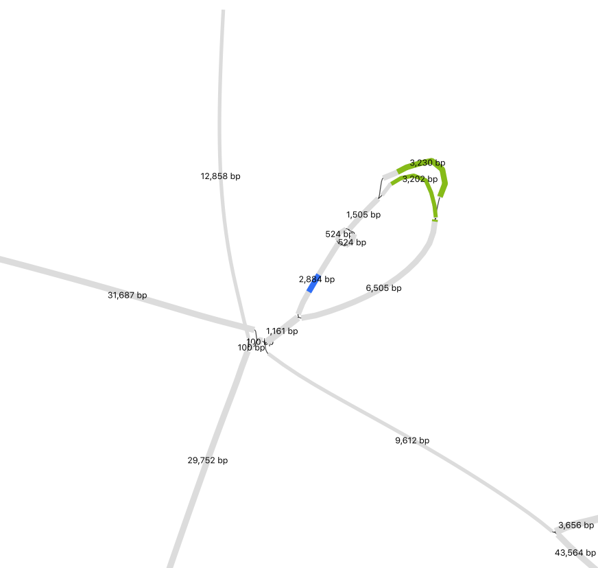
In late 2016, I was excited. I had observed (Barnum et. al 2018) that a set of simple communities enriched from bay mud contained abundant bacteria from the Candidate Phyla Radiation (CPR) and an abundant archaeum from the DPANN superphylum. CPR and DPANN organisms may form large portions of the tree of life and share a strange biology: they are obligate epibionts of other cells. The lifestyle of these symbionts may teach us more about microbial biology and ecology, their parasitism of other cells may be exploited as biocontrol agents, and the way they form connections between cells could be translated into biotechnology. And – at that point – had only been isolated in co-culture 5 times. Here were several of these enigmatic organisms, sometimes among the top 10 most abundant genomes in a community.
I thought, what if I could find a way to isolate these organisms in co-culture? Being well-versed in how targeted cultivation can fail from teammates’ experiences in my lab, I wondered if there were ways to do so in an untargeted, scaleable way.
I devised a promising approach, spoke with a professor on campus who was an expert on these organisms, gathered some simple laboratory supplies, and self-assuredly struck out to isolate the CPR and DPANN. Unfortunately, a third-year PhD student with a good idea has no power to achieve it without support from supervisors and funders, and I failed to win that support. I stopped my attempt, returned to my dissertation research on chlorine, and started pushing my one good idea on others at UC Berkeley. (Like a normal grad student, I did so merrily at seminars and grumpily at happy hours). I thought I should share this idea more broadly, but I worried doing so before could have interfered with others’ research.
Now, the field has reached a turning point where many groups have had recent success cultivating these small, epibiotic microorganisms. In particular, Batinovic et. al 2021, discussed below, showed me that “the cat is out of the bag.” I bet that several research groups have co-cultured isolates awaiting publication. I expect that similar ideas have been discussed in groups at conferences. I hope that other groups have considered / are implementing what I will suggest here and will succeed soon. (If you are reading this: don’t worry, no one will scoop you because of this blog post! You got this!). All of this is to say that I don’t view this as an original insight. I am no longer employed at an academic institution but still consider myself part of the community, and I think my community would benefit from having a more open discussion about this interesting cultivation problem.
The Standard Approaches
It is ridiculous to call the successful isolation of a hard-to-isolate organism as “standard,” as it is nothing but herculean or inspired or (as you will see in some cases) flat-out lucky. That being said, these are the approaches that have thus far been successful, in reverse chronological order, to my knowledge:
Batinovic et. al 2021 (behind the paper) applied filtered wastewater fluid onto plated lawns of Gordonia amarae (phylum Actinobacteria) and whole-genome sequenced clear plaques that formed on those lawns. Many of the plaques were bacteriophage, but one of the plaques was Candidatus Mycosynbacter amalyticus (phylum: Saccharibacteria / fmr. TM7).
Moreira et. al 2021 (behind the paper) used a micromanipulator attached to a light microscope to physically pick an epibiont, Vampirococcus lugosii (phylum: Absconditabacteria / fmr. SR1), and its host, a Halochromatium-related species (phylum: Proteobacteria), from a lake water culture enriched for anoxygenic phototrophs. They then sequenced the organisms.
Hamm et. al 2019 enriched and isolated Halorubrum lacusprofundi strain R1S1 in hypersaline water, later detecting a Nanohaloarchaeum in metagenomes of the enrichment culture. Fluorescence activated cell sorting of Ca. Nanohaloarchaeum antarcticus (phylum: Nanohaloarchaeum) from the enrichment allowed for its reliance on its host to be confirmed.
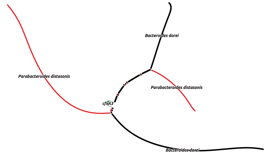
Cross et. al 2019, rather remarkably, used proteins encoded in TM7 cells (phylum: Saccharibacteria / fmr. TM7) to create antibodies that could selectively capture these organisms and their hosts (various Actinobacteria), which were subsequently plated.
Golyshin et. al 2017 with sequencing identified Candidatus Mancarchaeum acidiphilum (phylum: Micrarchaeota) in a culture of the acidophile Cuniculiplasma divulgatum (phylum: Thermoplasmatota).
St. John et. al 2017 used qPCR to monitor enrichments for Nanoarchaea, having a breakthrough when adding 0.22-micrometer filtrate into defined cultures of isolates, upon which they obtained a stable enrichment of Ca. Nanoclepta minutus (phylum: Nanoarchaeota) and its host Zestosphaera tikiterensis (phylum: Crenarchaeota).
Wurch et. al 2016 also used qPCR to monitor enrichments for Nanoarchaeota, followed by optical tweezer selection of a single host-epibiont pair, a successful hyperthermophilic and acidophilic co-culture of Ca. Nanopusillus acidilobi (phylum: Nanoarchaeota) and its host Acidilobus sp. 7A (phylum: Crenarchaeota).
He et. al 2015 enriched for Nanosynbacter lyticus TM7x (phylum: Saccharibacteria / fmr. TM7) using antibiotics and only detected it with PCR in plated colonies with Actinomyces odontolyticus XH001 (phylum: Actinobacteria). The connection between cells was apparent with light microscopy. See Utter et. al 2020 (behind the paper) for an important follow-up.
Huber et. al 2002 observed under a light microscope that a hyperthermophilic “isolate” (nice try!) of Ignicoccushospitalis (phylum: Crenarchaeota), obtained from a shallow marine hydrothermal vent, was covered by Nanoarchaeum equitans (phylum: Nanoarchaeota).
Guerrero et al. 1986 originally described Vampirococcus (phylum: Absconditabacteria / fmr. SR1) after observing it with light microscopy attached to Chromatium (phylum: Proteobacteria) cells in environmental samples, which inspired Moreira et. al to carry out their study, but its special evolutionary position would not be recognized until this year.
By my count, these incredible successes have resulted in the following number of species:
CPR Bacteria: 5 Saccharibacteria and 2 Absconditabacteria.
DPANN Archaea: 3 Nanoarchaeota and 1 Nanohaloarchaeum.
The isolations fall into several categories:
Serendipitous: observation of an epibiont with an already isolated host (e.g. Huber et. al).
Casual: identification of an epibiont with a host, and a subsequent pain-free isolation (e.g. Moreira et. al).
Targeted: purposeful co-cultivation of an epibiont and host, often with many attempts (e.g. St. John et. al).
Targeted, made easier by expensive investment: development of a method to selectively pull an epibiont and host into isolation (e.g. Cross et. al).
Should others try to reproduce these methods? If researchers take the extra step to look for epibionts while isolating other strains, “casual” isolations should increase. And by all means, go have a “serendipitous” discovery. Unfortunately, all of the “targeted” methods share a big drawback: intense effort focused on a single host or epibiont. We should admire these researchers’ effort and success while asking:
Is there a better way?
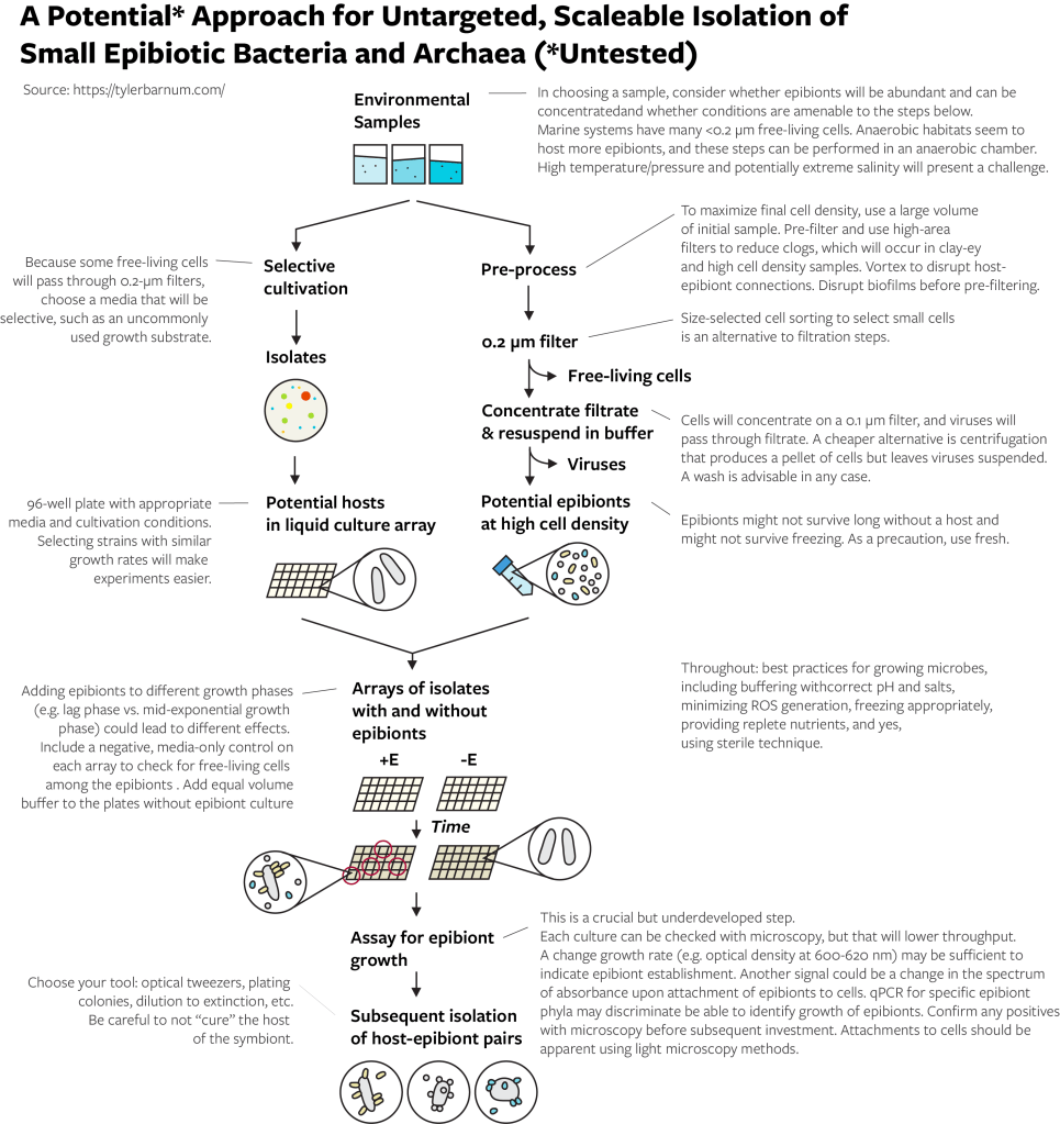
A Potential Untargeted, Scaleable Approach
Consider Batinovic et. al 2021 from a different perspective. From a habitat filled with many different epibiotic species and many host species, they (1) isolated a potential host, (2) selected all potential epibiotic species (with a 0.2-micrometer filter), (3) re-introduced those potential epibiotic species to the isolated potential host species, (4) watched for changes in the isolate that indicated the colonization of the isolate by an epibiont, and (5) confirmed the colonization of the epibiont.
You will, I expect, immediately ask yourself a series of questions:
What if you repeated the process but with a different potential host?
What if you repeated the process but with 100 different potential hosts?
What if you repeated the process but with epibionts collected from many samples from the same habitat?
How many more hosts and epibionts could you find?
The sum answer to these questions it that there is no reason to think that by scaling the isolation process and not focusing efforts on a single targeted host or epibiont, you would dramatically increase the likelihood that you obtain epibionts in co-culture.
Let’s consider there is a probability that a isolatable bacterium or archaeum could be a host of a epibiont present in its habitat (P_host), a probability that a epibiont among a sample could be cultivated (P_epibiont), and a probability that the colonization of the host by the epibiont can be observed (P_observation). What is the probability that you can get the epibiont in co-culture (P_get_epibiont_for host)? Perhaps a reasonable set of assumptions – that hosts are relatively rare, that a epibiont for that host won’t always be present in a community, and that an assay for observation would miss half of cases – the probabilities would be P_host = 0.1, P_epibiont = 0.2, and P_observation = 0.5. The joint probability would be P_get_epibiont_for host = P_host * P_epibiont * P_observation = 0.1 * 0.2 * 0.5 = 0.01. So, you have a 1 in 100 chance of getting a epibiont for a single potential host. But if you try 100 potential hosts, according to the binomial distribution, your probability of a 0 success is P_failure = (100!/ 0! (100-0)!) * (P_get_epibiont_for)^0 * (1-P_get_epibiont_for)^(100-0) = 0.37, or about 2 in 3 chance of success. Not bad! For 1000 potential hosts, with a naive assumption of the probabilities being independent, the probability of 0 successes is miniscule (0.0001).
My thinking on how to do this has not changed much over the years. I believe that these steps will work but encourage you to reevaluate them:
Choose an appropriate habitat.
Isolate many potential hosts.
Select potential epibionts by cell size, removing viruses and free-living cells as much as possible, and concentrate.
Grow host cultures with and without the addition of the epibiont concentrate.
Assay for the growth of epibionts with the host. Confirm with microscopy.
Isolate specific host-epibiont pairs.
How you implement these steps depends on your available equipment and your ability to increase throughput. The below method flowchart provides some suggestions and important notes. I played around with this enough in 2017 (very little) to know that the size selection and assay for epibiont growth are important steps to get right. For example, you need to use a filtration set up that will not get clogged by large volumes of liquid. For another example, if your assay is microscopy, looking at a microscope over and over again will take a lot of time. For yet another example, contrary to common opinion, free-living cells can and will pass through 0.2-micrometer filters (especially certain marine bacteria), so you should think about ways to limit their growth with a selective growth medium. Equipment to sort cells by size is not widely available but may be a huge benefit for the initial collecting of epibionts and for finding and collecting host cells to which epibionts are attached.
A note on habitat and host strains. Everyone has a bias towards their familiar habitat or strain. I beg you, before you choose the same study system you have always worked with, consider how this will limit your likelihood of success. Have the presence of these organisms ever been demonstrated in your habitat of study? Do your host strains resemble wild strains, or have they been propagated in the laboratory for years? Please, be critical and set yourself up for success. As a default, I would suggest a highly connected habitat with high cell densities, fewer environmental filters, and moderate diversity. For example, saturated sediments from wetlands or streams would be a better place to start than agricultural soils or animal microbiomes. I know little about the biology of epibiotic microorganisms, but I presume they benefit from transport between hosts (hence highly connected, fewer filters) and a high availability of hosts (high cell density). Moderate diversity would seem to decrease the chance that a habitat has no cultivable host-epibiont pairs (i.e. low diversity) and the chance that the epibiont for an isolated host is at low relative abundance (i.e. high diversity). Avoid a community if you know that it only has one or two epibiont phylotypes because if there are only one or two hosts, you will likely not succeed in isolating either. If you have PCR primers for CPR or DPANN phylum of interest, testing a sample for a diverse set of these organisms using amplicon sequencing would be a smart check on your choice before additional work.
Why Has This Not Been Done Before?*
I don’t know.
I believe the description of some specific host-epibiont relationships has led to a feeling that host-epibiont pairs are rare and must be carefully teased out of a community. You must identify the host, with the epibiont, then isolate both. Some of the above papers make it clear that this is not the case in cultivation, or that an epibiont can be hosted by species from different genera. I do not argue that some or many epibionts can be specific to one host species. But assuming that even only a small fraction of epibionts have a very broad host range provides enough justification to pursue an untargeted approach by increasing P_epibiont in the above math.
I believe that microbiologists could more readily adopt higher-throughput approaches but may be constrained by what’s affordable or what’s familiar. (In some cases, the affordability concern continues the issue of valuing non-human resources over the time and output of very smart, talented, driven students and staff). Additionally, microbiologists who study epibionts may have invested time in learning metagenomics and be uncomfortable with investing more time learning cultivation methods, resulting in fewer researchers in this subject area working on cultivation.
Finally, I believe that these is a notion that uncultivated organisms must be fastidious, or hard to cultivate. In many cases, an organism may truly be fragile in cultivation conditions or reluctant to grow quickly. One can imagine how epibiotic bacteria and archaea could be slow to form attachments to their host, fail to have a growth rate equaling a fast growing host, etc. However, several of the above publications show that at sufficient cell densities, some epibionts can be removed from their host, filtered, and transferred to a different host, successfully! There is no reason to think these organisms are not robust and cultivable just because they haven’t been cultivated in large numbers. Instead of comparing them to uncultivated free-living cells, a more apt comparison would be to consider them like uncultivated phages: happy to proliferate when provided a suitable host.
So, while this cultivation strategy has not been done, I believe that it will work and provide easier access to study a unique type of biology.
* This phrasing was a bit of misdirection. Take note that the question should really be, “why has this not been done before at scale?” Batinovic et. al 2021 cultivated a Saccharibacteria organism with basically this approach. I am simply suggesting to do what they did, with more potential hosts and an approach tuned away from phages and towards epibiotic cells.
Happy cultivating, and good luck!
How should I cite this article?
You probably should not cite this article because it is a blog post. I did no publishable work, but if your research benefitted from this article, I would be pleased to see a mention in your acknowledgements section. I would most enjoy hearing how this helped you find something cool. I do not have any time to help because I spent it all on writing a blog post.
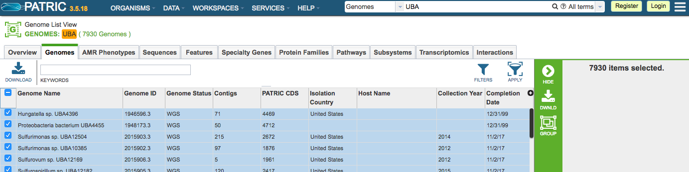
You are a student researcher and have identified an interesting protein with a fabulous function. You’d like to know what other organisms have this protein, and whether or not they are fabulous as well. However, the only tool you know of (yet) is the NCBI’s BLAST web server. The BLAST web server is very helpful and a good first stop. However, the BLAST web server:
Uses an algorithm that is bad at identifying proteins from the same clade that are highly dissimilar;
Can return pages of highly similar results if the gene has been sequenced in many organisms and you do not exclude the appropriate groups;
Does not provide an easy way, in my experience, to download genomes containing BLAST results.
Fortunately, you have other options.
Below are the databases that I tend to use, in order of their approachability to a researcher who is comfortable using command line tools and searching for proteins with HMMs (or command line BLASTP). I encourage you to learn how to use the command line (some resources here) and to build and use protein HMMs in your work. I detail some of this in a tutorial about searching large datasets. If you have not developed those skills yet, you have a different definition for which of these is approachable.
BLAST can help you identify the family your protein (or its domains) belongs to. From there, you can download various sets of proteins in the family and search for similar proteins on your computer. It is particularly useful to see if your protein groups with other proteins in a phylogenetic tree; you can then use a collection of proteins from a group to create a model (HMM) for your protein, aiding future searches.
EMBL-EBI’s hmmsearch allows you to search many databases, such as UniProtKB, using an HMM that you upload. (If you only have one protein and don’t want to build an HMM, phmmer is the tool for you). By adjusting reporting thresholds, you can limit the search to hits and use the convenient download options to collect similar proteins and their metadata.
A collection of proteomes representative of genetic diversity
Using “representative proteomes” [ref] is great if you to understand the distribution of your protein across the tree of life. The service grouped genomes by similarity at different levels, then selected a representative proteome (collection of proteins from the genome) for each group. For example, RP55 provides about one proteome per genus. The RPG file provides information about the proteomes, like strain name, that can be helpful in guiding your analysis. Also, since you have the entire proteome present, you can search for other proteins on the same set of organisms. Personally, I think this dataset is underutilized.
Note: if you want to visualize this distribution, the online tool AnnoTree is smartly designed to do just that.
Kai Blin’s tool for downloading genomes is not a database itself but a convenient and well-documented way to access RefSeq or GenBank. You can, for example, painlessly download all ~200 genomes in the genus Bradyrhizobium, then search those for, say, a chlorite:O2 lyase. Just be careful about data volume, particularly in highly sequenced lineages such as enteric pathogens. If you want, you can download all viral, bacterial, and archaeal genomes in RefSeq or GenBank.
IMG is like a great neighborhood bakery that only lets you buy one croissant at a time. I’m referring to the inability to search through >500 (meta)genomes at once (after you’ve create a Genome Set for those genomes), which I’m guessing was a conscious trade-off between better service for regular users and worse service for jerks trying to download the entire tree of life. (“Hurry up with my damn croissants!”). For our purposes, a clever workaround would be searching and downloading proteins annotated with a particular pfam, but many proteins belonging to a pfam lack the appropriate annotation. Not good if you want to identify new proteins.
Fortunately, you can use JGI’s instructions to download sequences (genomes, proteins, etc.) in bulk. The bulk download provides several files for each genome, including proteins (.faa), and is rather helpful. Note that according to a 2013 forum post, only genomes sequenced at JGI are available for download. Many of these genomes are not also uploaded into RefSeq or GenBank, so it can pay to search both if you want a full catalogue of available genomes.
What next?
Your choice of database and your analysis of it will depend on the scientific question you are trying to answer.
Often, I want to know where a group of new proteins fits into a preexisting tree, so I simply use a Pfam. For one project, I wanted to know the full extent of the gene’s diversity, so I searched pretty much every database. I also wanted to know what functions an accessory gene was involved in, so I used Python to parse genome files to get nearby genes (followed by many further analyses). For another project, I wanted to know if genes for a pathway were found together across the tree of life, so I used representative proteomes. If you are hesitant to learn programming (please don’t be!), some of this can be done on online web services for comparative genomics like IMG.
In my opinion, you’re likely looking for a protein because of its function, so when you consider its phylogenetic diversity you should also consider (1) the conservation of nearby genes that could be related in function and (2) the presence or absence of key residues, if they are known.
Get nearby genes (some Python helps) and seeing if they have homology using something like all-v-all comparisons or clustering. I use in-house scripts that I am still developing, but one published example of how this is done is here: https://github.com/ryanmelnyk/PyParanoid.
Create a protein alignment and compare positions to a characterized protein. Again, using Python can help, for example by using regular expressions to find the key positions.
Whatever you analysis is, you should validate your hits. Using a second technique to identify related proteins, such as building a phylogenetic tree, helps you remove false positives from a single technique alone.
Comparative genomics projects can be incredibly fun and can provide important insights, especially when you’re starting from a new protein. The projects have also been scary reminders of how diverse the microbial world is, and how much effort is needed to fully characterized it.
The following tutorials and documentation will be helpful for researchers considering similar approaches.
Using the command line
A command line enables you to perform diverse operations programmatically. That is, you can do a lot of things with it, and you can automate the process for easy repetition, alteration, and sharing. You should learn how to use a command line for bioinformatics. In fact, many bioinformatics programs are run not from a user interface but from the command line. Complicating things, the Windows command line uses its own language, whereas Mac and Linux machines, which use the Unix operating system, have command lines using more common bash language.
For Mac and Unix operating systems, use the local command line.
For Windows operating systems, you can try to use git bash (latest Windows) or Ubuntu. Ideally, you establish a remote connection (SSH) to a Unix operating system, perhaps a computer cluster maintained by your organization.
If you’re a Python novice, I encourage you to take a workshop and to use Python to analyze and plot your data, so you can get practice. These guides are helpful references and will expand your toolkit.
Python Data Science Handbook by Jake VanderPlas. Online Jupyter notebook with clear instruction and code examples, focused on different Python packages for data science (Jupyter Notebook, Numpy, Pandas, Matplotlib, machine learning with scikit-learn).
Metagenomics (assembly + genomics)
Going from sequencing to assembled genomes requires (1) assembly, (2) read-mapping, (3) binning genomes, and (4) bin refinement and quality check.
The iRep,EukRep, dRep, and dasTool suite of programs from the Banfield laboratory. iRep is a metric for replication rate. EukRep, dRep, and dasTool aide in binning and bin refinement.
CheckM is great for assessing genome completeness and contamination.
Running things on a laptop? Sickle for read trimming, MEGAHIT for assembly, and FastTree for tree-building – these programs are relatively fast compared to their peers.
Metagenomics (amplicon sequencing)
Current best practices are to remove sequencing errors from reads, obtaining amplicon sequencing variants (ASVs) instead of operational taxonomic units (OTUs). The DADA2 tutorial worked well for me.
Note: This is a tutorial for researchers new to studying large datasets of bacterial and archaeal genomes. It was originally written to specifically access the Uncultivated Bacteria and Archaea (UBA) dataset.
Outline
Introduction
Using HMMs to search a large dataset (Uncultivated Bacteria and Archaea (UBA))
New DNA sequencing and assembly technology provides researchers with more genomic sequences to explore than ever before. Any gene family is likely to be more diverse in metagenomes, which often contain uncultivated microorganisms, than in genomes from only cultivated microorganisms. Plus, when metagenomic sequences (“contigs” or “scaffolds” of contigs) have been sorted (“binned”) into genomes, the function and phylogeny of all genes in a microbial strain can be analyzed together. The discovery of bacteria that perform comammox (complete ammonia oxidation to nitrate) is a great example of this technology’s power.
The trouble in studying sequences from metagenomes is navigating databases that are both large and disparate. Metagenome-assembled genomes are distributed across the NCBI non-redundant protein sequences (nr) database, the Joint Genome Institute (JGI) Integrated Microbial Genomes (IMG) system, and the ggKbase system administered by Dr. Jill Banfield’s laboratory. Almost all published genomes an be found in the NCBI and/or IMG databases, and every system has a simple BLAST interface to quickly search for genes within genomes. Metagenomic sequences that have not been binned can be found in either the IMG (~10,000 metagenomes) or ggKbase (~1,000 metagenomes) databases. While a BLAST search can be performed on the entire NCBI nr and ggKbase databases, IMG limits BLAST searches to 100 genomes or metagenomes at once. Hopefully, researchers have provided annotated genomes on NCBI to be quickly queried, but sometimes they do not.
Unfortunately, one of the largest metagenomic datasets is not currently searchable. The Australian Center for Ecogenomics of the University of Queensland recently assembled and binned about 8,000 metagenome-assembled genomes from publicly available reads from over 1,500 metagenomes, which the authors refer to as the Uncultivated Bacteria and Archaea (UBA) genomes dataset. The UBA genomes substantially expanded the tree of life and may be a valuable resource for researchers who did not have the resources to obtain metagenome-assembled genomes from their datasets* or who want to perform comparative genomics of particular taxa across metagenomes.
Figure 1 from Parks et. al 2017 displaying the quality of ~8,000 UBA genomes assessed by CheckM
* That being said, assembling genomes from metagenomes is easier than ever and a great opportunity for students to learn programming skills that will benefit their data preparation and analysis in other areas. I hope that the strength of metagenomic super groups does not discourage other labs from adopting this technology or publishing reads along with their research.
While researchers can download UBA genomes from the NCBI BioProject (PRJNA348753) and annotate the genomes themselves, researchers cannot (yet*) search for genes in UBA genomes from any online portal. That is, good luck trying to find a UBA genome with an online BLAST search.
The best option available is to download UBA genomes or annotations from the author’s repository and perform a search on your computer. This tutorial describes how to do that: download and use Hidden Markov Models to search the UBA genomes for novel proteins. In theory, you can slightly alter this code to search through any number of genome annotations, such as a bulk download from JGI IMG.
Edit: An update on availability
I’ve been told that they will be uploaded to NCBI at some point, after which they will presumably be absorbed by IMG.
Additionally, Rob Edwards (UCSD) kindly informed me that the UBA genomes are available and searchable on PATRIC. My understanding is that with an account, PATRIC works similarly to IMG: word searches on all functional annotations and BLAST search on selected groups of organisms. The easiest way to search all UBA genomes is to search Genomes for “UBA,” select all, then select “Group.” You can know perform a BLAST search on the group. More documentation can be found on PATRIC’s online guide.
With other options available or at some point available, consider whether or not this below workflow is the best option for you to study UBA genomes. The transferrable skills from this tutorial are in searching any number of genomes for matches to a verified set of genes. I anticipate you will find the tutorial be a valuable for other datasets – I use these same techniques repeatedly in my own metagenome projects.
Searching the Uncultivated Bacteria and Archaea (UBA) dataset using HMMs
I use Hidden Markov Models (HMMs) and the program HMMER to search for new proteins because in my experience HMMs are better than BLAST at identifying sequences that have low percent identity but nevertheless belong within a group. BLASTP aligns short stretches of a single reference sequence to score new sequences according to their shared sequence identity and a matrix of values for different amino acids substitutions. HMMER uses a Hidden Markov Model, a statistical model trained on a set of reference proteins, to score new sequences. To understand the difference between the two techniques, consider two proteins that share 40-60% amino acid identity to a set of reference proteins, yet only one protein is within the phylogenetic clade of reference proteins. BLASTP will score both proteins similarly based on % amino acid identity. HMMER, which does not directly use % amino acid identity, will score the ingroup protein higher than the outgroup protein. Essentially, because HMMER uses statistical models of proteins, it is more robust against sequence variation. (BLAST is still great for identifying the most closely related sequences).
For this tutorial, I will be identifying chlorite dismutase (cld) from a reference set of experimentally confirmed proteins. Cld, and especially periplasmic Cld (pCld), catalyzes the degradation of toxic chlorite to choride and oxygen during the anaerobic respiration of perchlorate and chlorate to chloride, and it is rather oddly conserved among bacteria performing nitrite oxidation to nitrate. You can use your own protein (sub)family or perhaps the common phylogenetic marker for metagenomic assemblies, ribosomal protein subunit S3 (download a gapless FASTA for the pfam 00189 seed), which will be found in most of these genomes.
Necessary files
A FASTA format file of reference proteins ending in “.faa” (e.g. pcld.faa)
A FASTA format file of outgroup proteins ending in “-outgroup.faa” (e.g. pcld-outgroup.faa)
Download and unpack the UBA genomes first, since it takes about 3 hours to complete. If your computer memory is limited or your internet connection is poor, consider downloading the annotations divided into parts, which is explained in the final section of this post. For this tutorial I am only downloading the bacterial genomes, but you can perform this same analysis on archaeal genomes with minor changes to the code (it will probably work to Find and Replace “bacteria” to “archaea” then Find and Replace “bac” to “ar”).
# Download the "readme" file, which describes available files for download
wget https://data.ace.uq.edu.au/public/misc_downloads/uba_genomes/readme .

# Download annotations for all UBA bacterial genomes (archaeal genomes are a separate file)
# Size: 54 Gb, Runtime: ~90 minutes
wget https://data.ace.uq.edu.au/public/misc_downloads/uba_genomes/uba_bac_prokka.tar.gz .

# Unpack the tarball
# Size: 207 Gb, Runtime: ~90 minutes
tar -xzvf uba_bac_prokka.tar.gz

# Optional: remove unpacked tarball to save space
# rm uba_bac_prokka.tar.gz
While the genomes are being downloaded and unpacked, you may skip to “Build the Hidden Markov Model” below before returning to the next section.
Compile a single file of all proteins with headers identifying the source genome
Searching for proteins from UBA genomes is greatly simplified by combining all of the genomes’ proteins into a single file. However, it’s important to later be able to easily find proteins in their original genomes, but the headers do not clearly relate to a genome. The following for-loop command will concatenate all proteins while converting the protein headers to match its UBA genome:
# Before rename:
# Single proteome: UBA999.faa
# >BNPHCMLN_00001 hypothetical protein

# Concatenate renamed proteins into one file
# Size: 6.3 Gb, Runtime: ~5-10 minutes
for GENOME in `ls bacteria/`;
do sed "s|.*_|>${GENOME}_|" bacteria/${GENOME}/${GENOME}.faa | cat >> uba-bac-proteins.faa;
done

# After rename:
# All proteomes: uba-bac-proteins.faa
# >UBA999_00001 hypothetical protein

# Optional: remove all other files to save space.
# WARNING: Only do this if you're CERTAIN you do not need the files
# rm -r bacteria/
Build the Hidden Markov Model
After installing HMMER and installing muscle, you are ready to build a Hidden Markov Model from your reference set proteins. In constructing a reference set, select a set of proteins that is as broad as possible yet only includes verified proteins. Previous studies have used HMMs from published protein families (PFAM, TIGRFAM, etc.) and/or created their own custom HMMs (e.g. Anantharaman et. al 2016, available here). For reproducibility, I encourage you to published any custom HMMs and the sequences you used to construct them.
First, some organization. I find that it’s helpful to assign Unix variables so that code is completely interchangeable. I also suggest keeping a directory that contains all of your HMMs in one place (PATH_TO_HMM) as well as a directory that contains the reference sets (PATH_TO_REF). For this code to work, you need to edit the protein name and E-value threshold for each protein.
# Assign variable for protein name and E value threshold
# These should be the only variables you *have* to change for each protein

PROTEIN=pcld
E_VALUE=1e-50

# Assign variable for paths to reference protein sets and to HMMs
PATH_TO_HMM=HMMS
PATH_TO_REF=REFERENCE_SETS
REFERENCE=$PATH_TO_REF/$PROTEIN.faa
OUTGROUP=$PATH_TO_REF/$PROTEIN-outgroup.faa

# Create directories
mkdir $PATH_TO_HMM
mkdir $PATH_TO_REF
mkdir ./OUTPUT/
Now create the HMM.
# Change to the HMM directory
cd $PATH_TO_HMM
# Align reference proteins
muscle -clwstrict -in ../$REFERENCE -out $PROTEIN.aln;

# Build Hidden Markov Model
hmmbuild $PROTEIN.hmm $PROTEIN.aln

# Test your HMM by searching against your reference proteins
hmmsearch $PROTEIN.hmm $PROTEIN.faa

# Return to directory with UBA genomes
cd -
Search the UBA genomes using HMMER
The following is a simple HMMER search. You will need to calibrate the E-value (-E) or score (-T) cutoffs based on the quality and diversity of the reference set the HMM was trained on. We set those above when we indicated with protein ($PROTEIN) we’d be studying.
# Perform HMMER search using HMM and a threshold
HMM_OUT=./OUTPUT/table-${PROTEIN}.out
hmmsearch -E $E_VALUE --tblout $HMM_OUT $PATH_TO_HMM/$PROTEIN.hmm uba-bac-proteins.faa
The output contains the target name in the first column and the E-value and score in separate columns. All lines other than the targets start with a hash (#).
Results: HMMER identified 14 proteins above my threshold E-value for Cld. These proteins are very likely Cld and were even predicted as such by prokka (see: “description of target” at right). However, we know nothing else about these proteins without further analysis.
Save protein hits from UBA genomes
Identifying novel proteins is the goal but not the last step of analysis. You will likely want to create a FASTA file of your hits so that you can compare the new proteins to old proteins.
# Collect the headers of sequences above the threshold i.e. "hits" and sort
LIST_OF_HITS=./OUTPUT/hits-${PROTEIN}.txt
awk '{print $1}' $HMM_OUT > $LIST_OF_HITS
sort $LIST_OF_HITS -o $LIST_OF_HITS

# Optional: remove all lines with "#" using sed
sed -i 's/.*#.*//' $LIST_OF_HITS

# Collect proteins using headers
# Perl code from: http://bioinformatics.cvr.ac.uk/blog/short-command-lines-for-manipulation-fastq-and-fasta-sequence-files/
HITS=./OUTPUT/hits-${PROTEIN}.faa
perl -ne 'if(/^>(\S+)/){$c=$i{$1}}$c?print:chomp;$i{$_}=1 if @ARGV' $LIST_OF_HITS uba-bac-proteins.faa > $HITS
Obtain metadata on UBA genomes of hits
Additionally, it’s helpful to know more about the genomes hosting the hits, which you can identify using the UBA ID we placed in the header of every protein in the dataset. Download Supplementary Table 2 (“Characteristics of UBA genomes”) and save it as a csv or download a copy from my github account (see: Outline).
# Create list of genome IDs appended with comma, de-depulicated, and first line removed
# Note: Any line not a full UBA ID like "UBA#####," will return extra results
LIST_OF_GENOMES=./OUTPUT/genomes-${PROTEIN}.txt
sed 's/_.*/,/' $LIST_OF_HITS > $LIST_OF_GENOMES
sort -u $LIST_OF_GENOMES -o $LIST_OF_GENOMES
echo "$(tail -n +2 $LIST_OF_GENOMES)" > $LIST_OF_GENOMES

# Create csv table of genome information from Supplementary Table 2
TABLE_OF_GENOMES=./OUTPUT/genomes-${PROTEIN}.csv
head -1 supp_table_2.csv > $TABLE_OF_GENOMES
while read LINE; do grep "$LINE" supp_table_2.csv >> $TABLE_OF_GENOMES; done <$LIST_OF_GENOMES

# You may open this in a table viewing software, or...
# View "UBA Genome ID," "NCBI Organism Name," "CheckM Completeness," "CheckM Contamination" (fields 2, 8, 5, and 6)
awk -F "\"*,\"*" '{print $2,$8,$5,$6}' $TABLE_OF_GENOMES
Results: Cld is present in 11 genomes in the genus Nitrospira (expected) and 1 genome in the order Gallionellales (unexpected!). The interesting genome, UBA7399 Gallionellales, is 79.3% complete and 1.46% contaminated, which is not great but not bad.
Align with reference proteins and build a phylogenetic tree
Before proceeding with your analyses, I highly suggest you create an alignment and phylogenetic tree to confirm the new proteins contain any key amino acids and have the correct phylogenetic placement. I open and view alignments and trees in graphical user interfaces, specifically AliView and MEGA.
# Align reference proteins with hits and outgroup proteins
# Note: Alignment is computationally intensive for longer/more sequences
ALL_PROTEINS=./OUTPUT/all-${PROTEIN}
cat $REFERENCE $OUTGROUP $HITS > $ALL_PROTEINS.faa
muscle -in $ALL_PROTEINS.faa -out $ALL_PROTEINS.aln

# Create tree (default settings for simplicity)
FastTree $ALL_PROTEINS.aln > $ALL_PROTEINS.tre

# Open and view the align with GUI software such as AliView
# Open and view the tree with GUI software such as MEGA
# Edit PDF in Adobe Illustrator or InkScape if you're fancy
Results: The alignment and tree are as expected. Cld from Nitrospira spp. group with Cld from previously sequenced Nitrospira. The Cld UBA7399_00885 from genome UBA7399 Gallionellales has lower sequence identity to other proteins but groups with Cld from characterized perchlorate- and chlorate-reducing bacteria, specifically those in the Betaproteobacteria (data not shown). I am assuming that Gallionellales strain is a (per)chlorate-reducing bacterium and will save its genome for later comparative studies.
Conclusions and Next Steps
With the above workflow, you have obtained:
An HMM model for searching proteomes
A list of protein hits above a significance threshold
Protein sequences for hits
Information on which UBA genomes contained hits
An alignment of hits with reference protein sequences
A phylogenetic tree of hits with reference protein sequences
Where you go from here depends on your scientific question. In most cases, you will save the specific subset of UBA genomes you’re interested in so that you can inspect those genomes further. You may want to confirm that genes on the same contig on your hit match the assigned phylogeny of the UBA genome.
For my analysis, it’s rather interesting that UBA7399 Gallionellales contains cld.A quick BLAST search of its ribosomal protein S3 sequence, found by a simple word search, supports its assignment in the Gallionellales, making it the first such taxon to contain cld. In a first, it contains no other known genes for perchlorate reduction, chlorate reduction, or nitrite oxidation, and the genes in close proximity to cld are not informative. However, my own research has encountered the widely known fact that horizontally transferred genes, such as those for perchlorate and chlorate reduction, assemble poorly from metagenomes, and the genome is only ~80% complete. It’s helpful to remember that the maxim “absence of evidence is not evidence of absence” is especially true in genome-resolved metagenomics.
Other Examples
I don’t intend to use any of the following data but want to show a couple of additional examples.
DsrA is half of the DsrAB dimer and essential for dissimilatory sulfate reduction, a widespread and important process. When using my dsrA.hmm and an E-value < 1e-100, the 7,280- genome bacterial UBA dataset contains 60 metagenome-assembled genomes with dissimilatory sulfite reductase, which are listed below. In comparison, the Anantharaman et. al 2018 paper identified dsrA in 123 metagenome-assembled genomes from over 4,000 genomes, including several phyla never before associated with dissimilatory sulfate reduction. One of those phyla, the Acidobacteria, is again represented here!
Cytoplasmic Nar nitrate reductase (cNarG) and periplasmic nitrate reductase (NapA)
Denitrification and dissimilatory nitrate reduction to ammonia are important processes in agriculture and just about any other system with active nitrogen redox cycling, and Nar and Nap are the primary nitrate reductases involved. A very quick glance (shows that many genomes in the UBA dataset have cnarG (776 genomes; E-value < 1e-200) or napA (361 genomes; E-value < 1e-200). This is a case where there are too many proteins to create a phylogenetic tree easily, so here’s a barplot:
Polyketide synthases
Polyketide synthases are important secondary metabolite biosynthesis proteins and tend to make the news when new ones are discovered. I very lazily copied the seed for pfam 14765, the polyketide synthase dehydratases, chose an arbitrary E-value threshold (< 1e-50) without verifying whether it was too low or too high, and aligned full-length PKS “hits” with the partial length pfam 14765 seed sequences, so this is not a correct analysis. But there are clearly polyketide synthases in the UBA dataset. Have fun!
Addenda: Limitations and Alternatives
EDIT: A proposal for the ethical use of this dataset
Upon reflection, I felt the need to add this section. Many researchers invested significant resources into sequencing metagenomes. I believe that while the UBA dataset has done a public service by assembling so many metagenomic reads that would never be assembled and binned, many metagenomic assemblies must have been published before researchers were ready to release them. This tutorial could accelerate the “scooping.” In your use of this dataset, please avoid using information from metagenomes that have not been published and state an intent to use similar data. For example, if you are studying nitrogenase genes and find a dataset rich with interesting nitrogenase genes, I argue that it is unethical to include those genes in your analysis if the metagenome’s stated purpose is to study nitrogenases – unless they’ve already published the work. Maybe you disagree. But would you want someone to steal your dissertation research? Obviously not.
How to find this information (using the Cld example):
Find the SRA accession in the field “SRA Bin ID” (e.g. SRX332015);
Select “BioProject” from the “Related Information” panel on the right (e.g. PRJNA214105);
Inspect the description of the BioProject (e.g. no information makes me concerned about using Cld sequences or a single genome from this sample).
Record which BioProjects you can use and the SRAs belonging to them.
Script
I have created a bash script, available on github, to run all of the above code after the download and preparation of the UBA bacterial dataset. Edit the path to your HMMs and reference proteins in the script, then run using the following command:
sh uba-hmmer-pipeline.sh <protein> <E-value threshold>
Low memory
If you do not have a computer cluster or hard drive with enough memory to handle the 267 Gb total created by this workflow, you should consider downloading and processing the dataset in parts.
Try this nested for-loop, which should create no more than ~65 Gb at any one time and result in a ~7 Gb FASTA file of proteins. I did not test this, and you will probably need to change the directory “bacteria” to the directory created by unpacking the download in parts. You may find it easier to download one at a time manually.
# For parts 00 through 05
for NUM in 00 01 02 03 04 05;
do

# Download annotations for all UBA bacterial genomes
wget https://data.ace.uq.edu.au/public/misc_downloads/uba_genomes/uba_bac_prokka.part-$NUM . ;

# Unpack the tarball and promptly remove it to save space
cat uba_bac_prokka.part-$NUM | tar xz
rm uba_bac_prokka.part-$NUM

# Collect proteins
for GENOME in `ls bacteria/`;
do
sed "s|.*_|>${GENOME}_|" bacteria/${GENOME}/${GENOME}.faa | cat >> uba-bac-proteins.faa;
done

rm -r bacteria/

done
Searching for nucleotides or other information in genomes
The above tutorial covers searching for proteins, but you can easily search this dataset for genes in nucleotide sequences, for example, using BLASTN directed at *ffn files. The available genome annotations are standard output from prokka:
.gff This is the master annotation in GFF3 format, containing both sequences and annotations. It can be viewed directly in Artemis or IGV.
.gbk This is a standard Genbank file derived from the master .gff. If the input to prokka was a multi-FASTA, then this will be a multi-Genbank, with one record for each sequence.
.fna Nucleotide FASTA file of the input contig sequences.
.faa Protein FASTA file of the translated CDS sequences.
.ffn Nucleotide FASTA file of all the prediction transcripts (CDS, rRNA, tRNA, tmRNA, misc_RNA)
.sqn An ASN1 format “Sequin” file for submission to Genbank. It needs to be edited to set the correct taxonomy, authors, related publication etc.
.fsa Nucleotide FASTA file of the input contig sequences, used by “tbl2asn” to create the .sqn file. It is mostly the same as the .fna file, but with extra Sequin tags in the sequence description lines.
.tbl Feature Table file, used by “tbl2asn” to create the .sqn file.
.err Unacceptable annotations – the NCBI discrepancy report.
.log Contains all the output that Prokka produced during its run. This is a record of what settings you used, even if the –quiet option was enabled.
.txt Statistics relating to the annotated features found.
.tsv Tab-separated file of all features: locus_tag,ftype,gene,EC_number,product
Incomplete genomes
Most of the metagenome-assembled genomes from the UBA dataset are less than 90% complete, which means they seem to be less complete than most closed genomes. As noted above, this can lead to the absence of important genes that can inform your analysis. Also, here’s how the assembly of UBA genomes is described in the methods:
Each of the 1,550 metagenomes were processed independently, with all SRA Runs within an SRA Experiment (that is, sequences from a single biological sample) being co-assembled using the CLC de novo assembler v.4.4.1 (CLCBio)
That is, single samples were used for assembly and binning. It’s known that assembling reads from multiple samples can improve the assembly of rare genomes and deteriorate the assembly of common genomes. It’s also known that differential coverage information – reads mapped from multiple samples with varying strain abundances – improves binning. In summary, it’s likely that many bins could be improved through more careful binning of a few samples. You can try to assemble and bin these genomes yourself using Anvi’o.
Genomes without protein annotations
You can obtain structural annotations for any genome sequence quickly using prodigal, which is the backbone of prokka.
prodigal -i genome.fna -a proteins.faa -d genes.ffn
Other datasets
Obviously, you might be more interested in other sets of genomes. I provide some options in another tutorial here.
Citations
UBA genomes:
Parks DH, Rinke C, Chuvochina M, Chaumeil P-A, Woodcroft BJ, Evans PN, et al. (2017). Recovery of nearly 8,000 metagenome-assembled genomes substantially expands the tree of life. Nat Microbiol2: 1533–1542.
Other genome-resolved metagenomics papers demonstrating some useful practices. Disclosure: I work closely with the Banfield lab, and one of these papers is my own.
Anantharaman K, Hausmann B, Jungbluth SP, Kantor RS, Lavy A, Warren LA, et al. (2018). Expanded diversity of microbial groups that shape the dissimilatory sulfur cycle. ISME J. e-pub ahead of print, doi: 10.1038/s41396-018-0078-0.
Anantharaman K, Brown CT, Hug LA, Sharon I, Castelle CJ, Probst AJ, et al. (2016). Thousands of microbial genomes shed light on interconnected biogeochemical processes in an aquifer system. Nat Commun7: 13219.
Barnum TP, Figueroa IA, Carlström CI, Lucas LN, Engelbrektson AL, Coates JD. (2018). Genome-resolved metagenomics identifies genetic mobility, metabolic interactions, and unexpected diversity in perchlorate-reducing communities. ISME J12: 1568–1581.
Crits-Christoph A, Diamond S, Butterfield CN, Thomas BC, Banfield JF. (2018). Novel soil bacteria possess diverse genes for secondary metabolite biosynthesis. Nature558: 440–444.
Note: This is a tutorial to help other microbiologists learn a research method from a recent publication (EDIT: open-access PDF). This method can be applied to de novo genome and metagenome assemblies from short read sequencing data (e.g. Illumina) but is not relevant for assemblies using long read sequencing data (e.g. PacBio).
Code In Brief
As the below article details, I recommend that all genome-resolved metagenomic studies use Bandage to inspect assembly graphs, at a minimum, to check for (1) abundant genomes that have been critically mis-assembled and (2) genes crucial to your study that may not have been binned.
The path to Bandage commands on a Mac is: /Applications/Bandage.app/Contents/MacOS/Bandage
Outline
Introduction
Preparing the Assembly Graph
Assessing and Improving Genome Binning
Recovering Specific Sequences
Future Directions and Lessons
Addendum: Alternatives
I. Introduction
The algorithms used to assemble genomes and metagenomes from short sequencing reads have a fundamental problem. When a genome contains two or more identical sequences, the algorithm will combine them into one consensus sequence instead of a producing unique contigs for every sequence. To show why this is an issue, consider what would happen if an algorithm, set to use 5-letter substrings, assembled the following sentence:
“Everything is everywhere but the environment selects.” (depth=1x)
Because the substring “every” appears twice, the assembly algorithm combines them as a consensus sequence. Consequently, the algorithm cannot determine the correct order of the sequences. The result is a fragmented sequences, with the repetitive sequence as the point of fracture:
“Every” (2x)
“thing is” (1x)
“where but the environment selects.” (1x)
Clearly, much of the meaning is lost. (Though some would argue the meaning of the sentence has been improved).
Although genome assemblies involve nucleotides and longer substrings than the example above, they suffer from the same flaw: a repetitive sequences will fragment one long sequence into several smaller sequences. Metagenome assemblies are extra complicated because related microbes can have mostly, but not entirely, identical genomes, creating mis-assemblies caused by what I will refer to as “strain variation.” The combination of repetitive sequences, caused by duplication and horizontal transfer, and strain variation, caused by conserved sequences amid varying sequences, presents two major issues for metagenome assembly. First, the mis-assembly of specific sequences which limits recovery of important genes, like the highly conserved gene for 16S ribosomal RNA. Second, the fragmentation of genomes into many smaller contigs, which limits genome recovery using assembly and binning. These issues are related – what is genome fragmentation but the mis-assembly of many sequences? – but pose different problems for different analyses.
Assembly graphs, also known as contig graphs and de Bruijn graphs, can help remedy the problems posed by mis-assembly. Analyzing assembly graphs with a tool such as Bandage (a Bioinformatics Application for Navigating De novo Assembly Graphs Easily) [1] provides crucial context for correcting mis-assemblies in a simpler format than read-mapping, a complementary tool. As shown in the below video, with assembly graphs you can quickly intuit the quality of the assembled genome and methodically diagnose mis-assemblies, such multiple copies of the 16S rRNA gene interfering with one another’s assemblies.
In a recent publication [2], I used assembly graphs of a metagenome assembly to fix mis-assembled sequences and assign them to “bins,” the collections of contigs constituting a metagenome-assembled genome. Because these mis-assembled sequences were the primary subject of the research, the publication of the study absolutely depended on assembly graphs for the recovery of the sequences. Your needs may not be as dire, but assembly graphs could still prove useful. Below, I use the published data to describe how to recover specific sequences and assess genome binning quality, which was not detailed in the publication but is likely to be helpful in almost any metagenome study.
First, a little background on the research. I study a metabolism called perchlorate reduction, in which bacteria use a modified electron transport chain to respire perchlorate (ClO4-). (How and why some bacteria get their energy from perchlorate, which rains down from the atmosphere in only the tiniest amounts, is fascinating, understudied, and not at all relevant here). Only isolated perchlorate-reducing bacteria have been studied, so not much was known about the diversity of uncultivated perchlorate reducers and how they might interact with other organisms. By performing metagenome sequencing on communities fed perchlorate, I hoped to find out which microbes reduced perchlorate and which did something else. The only problem? The genes for perchlorate reduction, perchlorate reducatase (pcr) and chlorite dismutase (cld), are horizontally transferred, so different organisms possessed highly similar sequences of the same genes. As you can now predict, most copies of pcr and cld were divided between short contigs and impossible to accurately bin – a far too common problem in metagenomic datasets.
II. Preparing the Assembly Graph
Limitations and Strategies
Before you attempt to use assembly graphs in metagenomics, please note that currently, it is very hard to work with larger metagenomic datasets. Ryan Wick, the developer of Bandage, provides some helpful tips for dealing with large metagenomic datasets that you should read fully. I have been able to apply this technique to a metagenome of about 80 recovered genomes and 1,000 Mbp total sequence (2.6 Gb file, unpublished results), but it was exceptionally slow and frustrating. I predict that for any metagenome with >40 recovered genomes, reducing the dataset’s complexity will greatly improve the speed and utility of your assembly graphs analysis.
One strategy to reduce the complexity of the metagenomic dataset is to assemble each sample independently. Most metagenome assemblies combine all reads to increase coverage, but assembling samples individually provides its own advantages. Specifically, it both reduces the total size of each assembly (increasing Bandage’s speed) and, importantly, decreases the likelihood that a closely related genome/sequence is present (lowering the chance of mis-assembly). The cost is in coverage (fewer genomes recovered) and, in some cases, time and memory required to analyze samples one-by-one. A compromise would be to assemble similar samples together.
A complementary strategy is to subsample reads prior to assembly. Essentially, selecting a subset of reads filters out low-abundance genomes that create mis-assemblies from strain variation. The downside is that perfectly fine, less-abundant genomes are also removed. seqtk has a convenient subsampling tool.
# Subsample 1% of reads to a new file
SUB=0.01
RANDOM_STRING=100
seqtk sample -s $RANDOM_STRING f.fastq $SUB > ${SUB}_f.fastq
seqtk sample -s $RANDOM_STRING r.fastq $SUB > ${SUB}_r.fastq
Note: if you do use either of these strategies to assist with genome binning, you can use dRep to de-replicate the genomes recovered from multiple assemblies. (dRep was developed by my colleague, Matthew Olm).
A final simple strategy to reduce the complexity of the graph is to run the Bandage “reduce” command from a command line (not available within the GUI). This command subsamples the assembly graph according to specific parameters, including contigs/nodes within a certain range of read depth (caution: within-genome variation can be rather large) or within a certain distance from a BLAST hit or node of interest (caution: at high distances, e.g. >20, this can capture multiple genomes). Using a reduced graph will quickly and painlessly improve Bandage’s performance but will not correct any inherent issues in the assembly arising, for example, from strain variation.
Try a total assembly yourself, then see if you need to take extra measures to reduce the datasets’ complexity.
Creating the Assembly Graph
Bandage supports assembly graphs produced by several different assemblers (see: supported formats). I used MEGAHIT (FASTG format), which requires an additional command after assembly to generate the assembly graph. For example:
# Trim reads prior with Sickle
sickle pe -f f.fastq -r r.fastq -t sanger -o f_trimmed.fastq -p r_trimmed.fastq -s singles_trimmed.fastq q=20

# Assembly
megahit -1 f_trimmed.fastq -2 r_trimmed.fastq -o output
# MEGAHIT also has presets for different types of metagenomic datasets
# After assembly
cd output/intermediate_contigs
megahit_toolkit contig2fastg 99 k99.contigs.fa > k99.fastg
open k99.fastg
Bandage developers have supplied a sample genome assembly to inspect. If you would like to try out using assembly graph on a metagenomic dataset, you can download, trim, and assemble reads from a simple, 4-genome community observed in my study.
Scaffolding vs. Assembly Graphs
Scaffolding is a method to extend and combine contigs that produces more-complete metagenome-assembled genomes. Assembly graphs, however, are composed of contigs, not scaffolds. If you would like to use assembly graphs from a metagenomic dataset that has been scaffolded, you must parse your scaffolding output to find the contigs within each scaffold withineach bin. How to find and parse this information will vary by scaffolding method. (For the scaffolding algorithm SSPACE, the relevant information is in the files “*.final.evidence” and “*.formattedcontigs_min0.fasta”). If you’re bold, you may skip scaffolding, which has worked for me on very enriched communities with fewer genomes and less strain variation.
III. Assessing and Improving Genome Binning
Visualizing assembly graphs allows you to quickly and qualitatively understand your assembly in ways that simple metrics such as N50 and total size cannot.
An assembly graph of the combined assembly of five samples, totaling 612 Mbp, 746,102 nodes, and 146,832 edges.
Aside from a quality check on assembly, it can also assist in binning metagenome-assembled genomes. How? More-abundant genomes tend to have contigs linked to one another spatially in the graph. Because you’re a human and remarkable at recognizing patterns, you can use assembly graphs to:
Include sequences too short for binning algorithms (<2000-2500 bp).
Include sequences of too aberrant coverage for binning algorithms (e.g. rRNA genes)
Identify misbinned sequences within a contiguous assembly.
Identify strain variation in abundant genomes, which can inform the subsampling of samples or reads.
In rare cases, create complete, finished genomes.
I’ll explain each of these uses below. First, some basics. You can highlight a specific bin by selecting its contigs/nodes:
# Create list
BIN=bin001
grep '>' ${BIN}.fasta > ${BIN}.headers.txt # Select contigs
sed 's/>k99_//' ${BIN}.headers.txt > ${BIN}.nodes.txt # Remove prefix
sed -i 's/$/,/' ${BIN}.nodes.txt # Add comma to end of line
# Copy and paste list into Bandage to color/label
More comprehensively, you can color and label many bins at once using a CSV file. Here are the specifications provided to me by Ryan Wick:
The feature currently works as follows: if a column in your loaded CSV file has a header of “color” or “colour” (case insensitive), then the values in that column are treated as colours. The values can specify the exact colour, either as 6-digit hex (e.g. #FFB6C1), an 8-digit hex with transparency (e.g. #7FD2B48C) or a standard colour name (e.g. skyblue). If the value does not fit any of those, then it is considered a category and assigned a colour automatically. All nodes with the same category will obviously get the same colour. These colours are assigned as the nodes’ custom colours, not as a new colour category.
For Anvi’o users, I have written a (novice) Python script that generates the CSV file for labeling bins. (EDIT: Antti Karkman at the University of Gothenburg has provided an edited script that for contigs that have been renamed and filtered using ‘anvi-script-reformat-fasta’). The script cycles through a limited set of 12 colorblind-safe colors, since people can only discriminate between 6-8 colors at once anyway. (I suggest that you focus in on closely related organisms, since those are more likely to be spatially adjacent in assembly graphs). The result is enlightening:
The combined assembly used in the publication [2]. Each of the 48 bins is one of 12 colors, every color is used 4 times. Unbinned sequences are in gray; these bins were below 70% complete (as assessed by CheckM) and not included in the publication.A different assembly from a well-sampled community that has undergone successive enrichments (unpublished data) and, accordingly, suffers less from strain variation. About 25 metagenome-assembled genomes were recovered. Only two suffer seriously from strain variation. Notably, this assembly did not require scaffolding. A MEGAHIT preset of meta-sensitive and final kmer size of 141 were used.
You can immediately notice which bins are near-complete with long, interrupted contigs and which bins have related genomes that interfered with assembly. If you did a good job binning, this image will be rather pleasing. It’s also a helpful educational display.
Even after rigorous binning, you can notice binning errors in the published dataset*; some sequences are indicated as unbinned (gray), probably because I excluded low quality bins from the analysis, and some bins have minor errors. Most researchers accept that any metagenome-assembled genome may have some contamination and that you cannot fix every error (one memorable quote: “you will get garbage from metagenomic assemblies”), but for those who seek be as rigorous as possible, as when identifying a new metabolism or a new phylum, this method will support your case. Below are some examples of common uses for assembly graphs in binning.
Include sequences too short for binning algorithms (<2000-2500 bp) & sequences of too aberrant coverage for binning algorithms (e.g. rRNA genes)
The short and/or abundant sequences could have been binned with the surrounding bin.
To include all nodes that are contiguous with a genome bin, you can create a reduced graph extended from the binned contigs. Be aware that some bins can be connected to dozens of others, so you should be selective.
# Remove new line characters from list of nodes
tr -d '\n' < bin001.nodes.txt > bin001.inline.nodes.txt

# Select all contiguous nodes to bin001
Bandage reduce k99.fastg bin001.gfa --scope aroundnodes --distance 50 --nodes `cat bin001.inline.nodes.txt`
# Load the Bandage GUI, load the CSV, and reinspect the bins
Identify misbinned sequences within a contiguous assembly.
The contigs in the red bin clearly belong in the purple bin. These errors become more common when strain variation is present, as indicated by the many breaks between contigs.
Identify strain variation in abundant genomes, which can inform the subsampling of samples or reads.
Genome BM101 was not happy to be assembled, likely due to the presence of multiple strains in the enrichment.
An important aside: While CheckM determined this bin to be 98% complete with 3% contamination, as judged by conserved single copy genes, we can clearly see that many accessory genes will be interrupted in or absent from the published metagenome-assembled genome. The true completeness of the genome was overestimated because the conserved sequences of the core genome were better assembled than variable genes. Additionally, binning tends to remove genes that have been adaptively gained or lost between samples. Together, this means that the estimated completeness of metagenome-assembled genomes is greater than that of the true genome.
Unfortunately, because strain variation is essentially the recreation of slightly diverged sequences, simply using Bandage to select all the contigs/nodes of a genome affected by strain variation can produce a genome bin with many more nucleotides and genes than the true genome. In this case, the completeness estimates may underestimate the genome’s duplicity. If strain 1 and strain 2 have very different coverage, a subsampling approach as discussed above may help disentangle one from the other. A fancier-though-not-always-better approach is to (1) select all of the contigs, (2) select all reads that mapped to those contigs from your BAM file, (3) subsample that subset of reads, and (4) assemble each subsampled subset. Decide before you start how desperate you are for a clean genome.
Strain variation can also be much more benign, as in the case of these genomes from the genus Denitrovibrio which are much more well-assembled and binned.
In my experience, strain variation is more likely to affect more-abundant genomes. There may be a biological reason for this, but it could simply be that less-abundant genomes do not have sufficient coverage of the minority strain to create an issue. For example, if two strains are in a ratio of 10:1 and a genome requires 4x coverage to assemble, assembly problems that are significant at 1000x coverage (1000x:100x) would be insignificant at 10x coverage (10x:1x) where the minority strain would not assemble by itself alone (1x < 4x).
In rare cases, create complete, finished genomes.
Manual assembly may have been to reduce this small CPR bacteria genome from 81 nodes to 8 nodes, which could then be scaffolded with manual read mapping.
The subsampling strategies discussed above are particularly useful for recovering complete genomes.
The Importance of Assessing and Improving Genome Binning
After completing a round of automated binning, you can assess your bins to an assembly graph to diagnose problems with binning such as strain variation and inaccurate binning. For example, in one metagenome assembly, strain variation so bad that the most abundant genome was undetected in binning because it was entirely fragmented into ~1000-bp contigs. After recovering a genome by assembling samples individually, the strain was found to have a key functional role! Highlighting bins in an assembly graph is one way to identify this example.
This metagenome assembly with about 80 genomes has abundant sequences that went unbinned (gray).The gray contigs, each of which has high read coverage but is ~1000-bp or less, should clearly have been assembled as one long contig. Instead, these sequences were filtered from the binning process.
Let this be a cautionary tale that you should at a minimum check a reduced assembly graph of the most abundant contigs for short, unbinned sequences.
# Select nodes >500x coverage and three connected nodes to maintain links
Bandage reduce k99.fastg graph.gfa --scope depthrange --mindepth 500.0 --maxdepth 1000000 --distance 3
Assembly graphs can improve most genome bins by capturing contigs too short or too aberrant in coverage. While this can consume as much time as you let it, you may be able to be more efficient and reproducible by automating processes. Alternatively, you can consider this a curation step for a genome(s) of special interest.
Note: For my publication, I relied exclusively on standard approaches for binning (i.e. Anvi’o), as most groups do, but the errors above indicate that bin recovery could have been improved by inspecting the assembly graph. Fortunately, none of the errors change the conclusions of the paper, but I still plan to update revised genomes to NCBI.
IV. Recovering Specific Sequences
Assembly graphs have a second important use: using qualitative information to assemble sequences that an algorithm cannot. Assembly graphs enabled me to manually assembly highly conserved sequences (16S rRNA genes) and horizontally transferred sequences (pcr and cld) that were crucial to my research. The goals are to merge short contigs belonging to a fragmented sequence and to link them to longer contigs that belong to genome bins. From the paper:
“Bandage . . . . was used to visualize contigs, identify BLAST hits to specific gene sequences, manually merge contigs, and relate merged contigs to a genome bin. Criteria for merging contigs were that contigs (1) shared a similar abundance and (2) lay in the same contiguous path. Merged contigs were binned when contiguity with multiple contigs from the same genome bin was certain. This strategy was also used to recover some 16S rRNA genes.”
This is particularly useful for unbinned contigs that, as you could notice in the above section, can be clearly linked to a specific genome.
Identifying and Visualizing Genes of Interest with BLAST
The first step is to identify the contigs/nodes that contain your gene of interest. You can either perform your own homology search or use the built-in BLAST annotation feature in Bandage (detailed instructions). While you may want to visualize all hits at first to understand the distribution among genomes, it is much simpler to reduce the Scope to “Around BLAST hits” or “Around [selected] nodes” and only show a short Distance of nodes. The key benefit? In a FASTA file all of these contigs appear are separate, yet in an assembly graph their spatial relationship is maintained.
Contigs/nodes adjacent to contigs with cld (blue) and pcr (green). Length in bp is indicated. These sequences were obtained from an individually assembled sample.
Manually Merge Contigs
In Preferences, adjust Depth and Node Width to accentuate coverage differences between nodes. This helps distinguish sequences from different organisms. To merge nodes, use Output > “Specific exact path for copy/save” to input selected node sequences. (Tip: Have a list of nodes, enter one at a time, and toggle +/- until Bandage confirms the path is possible). I only merged nodes if they share the same path (“contiguous”) and had logically similar abundance. In the below example, while at much higher abundance, the 1000x contig could be a duplicated sequence flanking the selected insertion and the sequences at the bottom left.
Manually merge contiguous contigs/nodes with equal coverage.
Remember that the sequence you recover is likely a consensus sequence. Usually, an assembler will use the higher coverage nucleotides to construct the contig, but in similarly abundant reads the result could be a mixture of nucleotide identities from two or more populations. If it matters for your study, you can perform an SNV analysis.
Relate Merged Contigs to a Genome Bin
Select a sequence from adjacent contigs and search for it among your bins. Often, as below with genomes “BM301” and “BM503,” the genome bin that the sequence of interest belongs to can be blindingly obvious: all contigs/nodes are contiguous and of similar abundance. (Note: reads can be recruited from similar sequences or unassembled sequences in your metagenome, distorting read depth).
Nodes 49954, 23972, 34899, and 15406 were binned in genome BM301. Nodes 49174 and 39643 were binned with genome BM503. Based on coverage and contiguity, nodes were either added to bin BM301 (orange), added to bin BM503 (blue), or added to both bins (gray). Contig 44798 is a transposase that flanks the transposon interior (right) and, accordingly, is found at twice the coverage.
From the paper:
A portion of the assembly graph (left) and the resulting annotation (right) for each selection, bin BM301 and bin BM503.
Other times, you will be less certain of the contiguity. It is best to conservative about merging and binning sequences. When necessary, you can use read mapping or even PCR to link some contigs to one another with more certainty.
Adding Sequences to Bins
Your manual assembly might include sequences that are already present in genome bins that should be removed from the genome bin before analysis. Duplicates contigs can be identified by the name of the contigs/nodes or, in the case of scaffolded sequences, by using nucmer:
This method enables you to recover and bin a consensus sequence from fragmented contigs. Crucially, with this manual assembly you can determine if more than one genome contains the same sequence. I understand any aversion to using this technique for that reason, but (1) ignoring something does not mean it is not there and (2) other techniques generate duplicity anyway, as evidenced for the need for programs like dRep.
Inspecting numerous assembly graphs has convinced me that many important gene sequences fail to be properly binned. At a minimum, I advise researchers search for connections between binned sequences and important genes that might be on unbinned sequences. You can either simply eyeball the size of the results or more accurately parse the returned contigs and compare that list to binned contigs. The following Bandage command enables such a search:
# Select portion of graph within 5 nodes BLAST hits to the key gene, with E-value filter of 1e-20
Bandage reduce k99.fastg reduced.gfa --query keygene.fasta --scope aroundblast --evfilter 1e-20 --distance 5
V. Future Directions and Lessons
Assembly graphs may only be useful for as long as de novo assemblies rely on short read sequencing. While in use, there is room for improved or alternative methods that are above my pay grade.
Code for updating an Anvi’o database/collection using revised binning selections from Bandage.
Automated refinement of binning by extending a bin’s graphs until it reaches another bin’s graph. This would allow binning to incorporate information from the assembler (note: this may not lead to improvements for all bins).
Using assembly graph information to assess completeness and contamination.
A complementary binning workflow for sequences less than <2500 bp that may constitute highly abundant genome(s) affected by strain variation. For example, all short contigs greater than 100x coverage are grouped by taxonomy. Contigs of a genome would be compared to BAM files to determine in which sample is coverage sufficiently highly and SNVs sufficiently low to enable assembly through subsampling.
Disentangling specific consensus sequences by using SNV coverage. For example, if 4% of sites in a sequence are variable because of two unique populations at ~10x and ~2x coverage, create two sequences using the (1) ~10x coverage SNVs and shared sites and (2) ~2x coverage SNVs and shared sites. If applied to entire genomes, this could be a potent way to fix strain variation.
What have I learned from using assembly graphs? Metagenomic datasets are tremendously valuable but also complex and fraught. The contigs output by the assembler often represent the composite of multiple strains as one genome. When the diversity among reads is sufficient enough, all or part of these composite genomes assemble poorly, destroying or dividing the genome. When gene gain or loss occurs between samples, genome binning tends to remove these accessory genes, which could very well be adaptive traits relevant to the study. Until the inherent issues are resolved by new comprehensive methods, researchers will be faced with making serious subjective decisions in the form of colorful spaghettis.
VI. Addendum: Alternatives
Of course, after submitting my paper and writing this blog, I found the publication describing MetaCherchant, a tool that reconstructs the genomic environment around a specific gene of interest. It is elegant, and I wish I had known about it, so I will highlight it here. MetaCherchant “builds a subgraph . . . around a target nucleotide sequence” and allows you to compare two samples to see if the genomic context of the gene has changed. MetaCherchant differs my the approach that I have described mostly in that (1) it builds a subgraph, not a graph of an entire metagenome, and (2) a specific gene of interest is used to build each graph, rather than observing multiple sequences in a single graph. Regardless, both approaches allow you to link a gene to genomes from a metagenome. Without having used the tool, I expect that MetaCherchant’s focused approach would afford some serious improvements in computational resources, time, and assembly quality if your goal is to analyze specific genes. The developers compared a total metagenome assembly from SPAdes to the localized metagenome assembly from MetaCherchant. The figure below, from their paper, shows that while the antibiotic resistance gene cfxA3 (green) to was successfully linked by both approaches (black) to the Bacteroides dorei genome, only MetaCherchant (red) linked cfxA3 to the Parabacteroides distasonis genome. That’s an important improvement in detection.
Are you instead looking for a programmatic way to improve binning? Check out Spacegraphcats, which finds groups of contigs in the assembly graph that, while hard to assemble into longer contigs, definitely belong together. Preprint here: https://www.biorxiv.org/content/10.1101/462788v1.
Ultimately, your goals and study design will inform the approach you choose.
Citing This Work
The following papers demonstrate Bandage [1] and the method and logic I used for using Bandage to recover specific sequences from metagenomic datasets [2]: