How to Search Large Sets of Genomes for Important Genes

Note: This is a tutorial for researchers new to studying large datasets of bacterial and archaeal genomes. It was originally written to specifically access the Uncultivated Bacteria and Archaea (UBA) dataset.

Outline

1. Introduction
2. Using HMMs to search a large dataset (Uncultivated Bacteria and Archaea (UBA))
3. Addenda: Limitations and Alternatives

Supporting files on github: https://github.com/tylerbarnum/metagenomics-tutorials

Introduction

New DNA sequencing and assembly technology provides researchers with more genomic sequences to explore than ever before. Any gene family is likely to be more diverse in metagenomes, which often contain uncultivated microorganisms, than in genomes from only cultivated microorganisms. Plus, when metagenomic sequences (“contigs” or “scaffolds” of contigs) have been sorted (“binned”) into genomes, the function and phylogeny of all genes in a microbial strain can be analyzed together. The discovery of bacteria that perform comammox (complete ammonia oxidation to nitrate) is a great example of this technology’s power.

The trouble in studying sequences from metagenomes is navigating databases that are both large and disparate. Metagenome-assembled genomes are distributed across the NCBI non-redundant protein sequences (nr) database, the Joint Genome Institute (JGI) Integrated Microbial Genomes (IMG) system, and the ggKbase system administered by Dr. Jill Banfield’s laboratory. Almost all published genomes an be found in the NCBI and/or IMG databases, and every system has a simple BLAST interface to quickly search for genes within genomes. Metagenomic sequences that have not been binned can be found in either the IMG (~10,000 metagenomes) or ggKbase (~1,000 metagenomes) databases. While a BLAST search can be performed on the entire NCBI nr and ggKbase databases, IMG limits BLAST searches to 100 genomes or metagenomes at once. Hopefully, researchers have provided annotated genomes on NCBI to be quickly queried, but sometimes they do not.

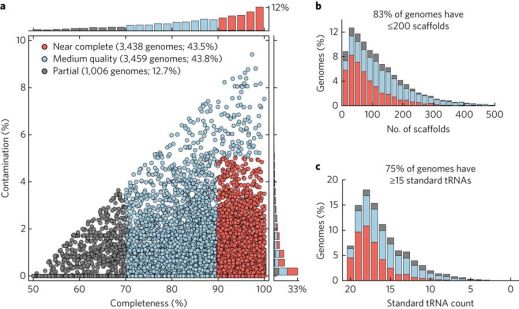
Unfortunately, one of the largest metagenomic datasets is not currently searchable. The Australian Center for Ecogenomics of the University of Queensland recently assembled and binned about 8,000 metagenome-assembled genomes from publicly available reads from over 1,500 metagenomes, which the authors refer to as the Uncultivated Bacteria and Archaea (UBA) genomes dataset. The UBA genomes substantially expanded the tree of life and may be a valuable resource for researchers who did not have the resources to obtain metagenome-assembled genomes from their datasets* or who want to perform comparative genomics of particular taxa across metagenomes.

* That being said, assembling genomes from metagenomes is easier than ever and a great opportunity for students to learn programming skills that will benefit their data preparation and analysis in other areas. I hope that the strength of metagenomic super groups does not discourage other labs from adopting this technology or publishing reads along with their research. 

While researchers can download UBA genomes from the NCBI BioProject (PRJNA348753) and annotate the genomes themselves, researchers cannot (yet*) search for genes in UBA genomes from any online portal. That is, good luck trying to find a UBA genome with an online BLAST search.

The best option available is to download UBA genomes or annotations from the author’s repository and perform a search on your computer. This tutorial describes how to do that: download and use Hidden Markov Models to search the UBA genomes for novel proteins. In theory, you can slightly alter this code to search through any number of genome annotations, such as a bulk download from JGI IMG.

Edit: An update on availability

I’ve been told that they will be uploaded to NCBI at some point, after which they will presumably be absorbed by IMG.

Additionally, Rob Edwards (UCSD) kindly informed me that the UBA genomes are available and searchable on PATRIC. My understanding is that with an account, PATRIC works similarly to IMG: word searches on all functional annotations and BLAST search on selected groups of organisms. The easiest way to search all UBA genomes is to search Genomes for “UBA,” select all, then select “Group.” You can know perform a BLAST search on the group. More documentation can be found on PATRIC’s online guide.

With other options available or at some point available, consider whether or not this below workflow is the best option for you to study UBA genomes. The transferrable skills from this tutorial are in searching any number of genomes for matches to a verified set of genes. I anticipate you will find the tutorial be a valuable for other datasets – I use these same techniques repeatedly in my own metagenome projects.

Searching the Uncultivated Bacteria and Archaea (UBA) dataset using HMMs

I use Hidden Markov Models (HMMs) and the program HMMER to search for new proteins because in my experience HMMs are better than BLAST at identifying sequences that have low percent identity but nevertheless belong within a group. BLASTP aligns short stretches of a single reference sequence to score new sequences according to their shared sequence identity and a matrix of values for different amino acids substitutions. HMMER uses a Hidden Markov Model, a statistical model trained on a set of reference proteins, to score new sequences. To understand the difference between the two techniques, consider two proteins that share 40-60% amino acid identity to a set of reference proteins, yet only one protein is within the phylogenetic clade of reference proteins. BLASTP will score both proteins similarly based on % amino acid identity. HMMER, which does not directly use % amino acid identity, will score the ingroup protein higher than the outgroup protein. Essentially, because HMMER uses statistical models of proteins, it is more robust against sequence variation. (BLAST is still great for identifying the most closely related sequences).

For this tutorial, I will be identifying chlorite dismutase (cld) from a reference set of experimentally confirmed proteins. Cld, and especially periplasmic Cld (pCld), catalyzes the degradation of toxic chlorite to choride and oxygen during the anaerobic respiration of perchlorate and chlorate to chloride, and it is rather oddly conserved among bacteria performing nitrite oxidation to nitrate. You can use your own protein (sub)family or perhaps the common phylogenetic marker for metagenomic assemblies, ribosomal protein subunit S3 (download a gapless FASTA for the pfam 00189 seed), which will be found in most of these genomes.

Necessary files

• A FASTA format file of reference proteins ending in “.faa” (e.g. pcld.faa)
• A FASTA format file of outgroup proteins ending in “-outgroup.faa” (e.g. pcld-outgroup.faa)

Dependencies

• Perl (preinstalled on Mac OS X; installation)
• HMMER (installation)
• MUSCLE (installation) or another sequence alignment software
• FastTree (optional; installation)

Download annotated UBA genomes

Download and unpack the UBA genomes first, since it takes about 3 hours to complete. If your computer memory is limited or your internet connection is poor, consider downloading the annotations divided into parts, which is explained in the final section of this post. For this tutorial I am only downloading the bacterial genomes, but you can perform this same analysis on archaeal genomes with minor changes to the code (it will probably work to Find and Replace “bacteria” to “archaea” then Find and Replace “bac” to “ar”).

# Download the "readme" file, which describes available files for download 
wget https://data.ace.uq.edu.au/public/misc_downloads/uba_genomes/readme . 

# Download annotations for all UBA bacterial genomes (archaeal genomes are a separate file)
# Size: 54 Gb, Runtime: ~90 minutes
wget https://data.ace.uq.edu.au/public/misc_downloads/uba_genomes/uba_bac_prokka.tar.gz . 

# Unpack the tarball
# Size: 207 Gb, Runtime: ~90 minutes
tar -xzvf uba_bac_prokka.tar.gz

# Optional: remove unpacked tarball to save space
# rm uba_bac_prokka.tar.gz

While the genomes are being downloaded and unpacked, you may skip to “Build the Hidden Markov Model” below before returning to the next section.

Compile a single file of all proteins with headers identifying the source genome

Searching for proteins from UBA genomes is greatly simplified by combining all of the genomes’ proteins into a single file. However, it’s important to later be able to easily find proteins in their original genomes, but the headers do not clearly relate to a genome. The following for-loop command will concatenate all proteins while converting the protein headers to match its UBA genome:

# Before rename: 
# Single proteome: UBA999.faa
# >BNPHCMLN_00001 hypothetical protein

# Concatenate renamed proteins into one file
# Size: 6.3 Gb, Runtime: ~5-10 minutes
for GENOME in `ls bacteria/`; 
do sed "s|.*_|>${GENOME}_|" bacteria/${GENOME}/${GENOME}.faa | cat >> uba-bac-proteins.faa; 
done

# After rename:
# All proteomes: uba-bac-proteins.faa
# >UBA999_00001 hypothetical protein

# Optional: remove all other files to save space.
# WARNING: Only do this if you're CERTAIN you do not need the files
# rm -r bacteria/

Build the Hidden Markov Model

After installing HMMER and installing muscle, you are ready to build a Hidden Markov Model from your reference set proteins. In constructing a reference set, select a set of proteins that is as broad as possible yet only includes verified proteins. Previous studies have used HMMs from published protein families (PFAM, TIGRFAM, etc.) and/or created their own custom HMMs (e.g. Anantharaman et. al 2016, available here).  For reproducibility, I encourage you to published any custom HMMs and the sequences you used to construct them.

First, some organization. I find that it’s helpful to assign Unix variables so that code is completely interchangeable. I also suggest keeping a directory that contains all of your HMMs in one place (PATH_TO_HMM) as well as a directory that contains the reference sets (PATH_TO_REF). For this code to work, you need to edit the protein name and E-value threshold for each protein.

# Assign variable for protein name and E value threshold
# These should be the only variables you *have* to change for each protein

PROTEIN=pcld
E_VALUE=1e-50

# Assign variable for paths to reference protein sets and to HMMs
PATH_TO_HMM=HMMS
PATH_TO_REF=REFERENCE_SETS
REFERENCE=$PATH_TO_REF/$PROTEIN.faa 
OUTGROUP=$PATH_TO_REF/$PROTEIN-outgroup.faa 

# Create directories
mkdir $PATH_TO_HMM
mkdir $PATH_TO_REF
mkdir ./OUTPUT/

Now create the HMM.

# Change to the HMM directory
cd $PATH_TO_HMM
# Align reference proteins
muscle -clwstrict -in ../$REFERENCE -out $PROTEIN.aln;

# Build Hidden Markov Model
hmmbuild $PROTEIN.hmm $PROTEIN.aln

# Test your HMM by searching against your reference proteins
hmmsearch $PROTEIN.hmm $PROTEIN.faa

# Return to directory with UBA genomes
cd -

Search the UBA genomes using HMMER

The following is a simple HMMER search. You will need to calibrate the E-value (-E) or score (-T) cutoffs based on the quality and diversity of the reference set the HMM was trained on. We set those above when we indicated with protein ($PROTEIN) we’d be studying.

# Perform HMMER search using HMM and a threshold
HMM_OUT=./OUTPUT/table-${PROTEIN}.out
hmmsearch -E $E_VALUE --tblout $HMM_OUT $PATH_TO_HMM/$PROTEIN.hmm uba-bac-proteins.faa

The output contains the target name in the first column and the E-value and score in separate columns. All lines other than the targets start with a hash (#).

Results: HMMER identified 14 proteins above my threshold E-value for Cld. These proteins are very likely Cld and were even predicted as such by prokka (see: “description of target” at right). However, we know nothing else about these proteins without further analysis.

Save protein hits from UBA genomes

Identifying novel proteins is the goal but not the last step of analysis. You will likely want to create a FASTA file of your hits so that you can compare the new proteins to old proteins.

# Collect the headers of sequences above the threshold i.e. "hits" and sort
LIST_OF_HITS=./OUTPUT/hits-${PROTEIN}.txt
awk '{print $1}' $HMM_OUT > $LIST_OF_HITS
sort $LIST_OF_HITS -o $LIST_OF_HITS

# Optional: remove all lines with "#" using sed
sed -i 's/.*#.*//' $LIST_OF_HITS

# Collect proteins using headers
# Perl code from: http://bioinformatics.cvr.ac.uk/blog/short-command-lines-for-manipulation-fastq-and-fasta-sequence-files/
HITS=./OUTPUT/hits-${PROTEIN}.faa
perl -ne 'if(/^>(\S+)/){$c=$i{$1}}$c?print:chomp;$i{$_}=1 if @ARGV' $LIST_OF_HITS uba-bac-proteins.faa > $HITS

Obtain metadata on UBA genomes of hits

Additionally, it’s helpful to know more about the genomes hosting the hits, which you can identify using the UBA ID we placed in the header of every protein in the dataset. Download Supplementary Table 2 (“Characteristics of UBA genomes”) and save it as a csv or download a copy from my github account (see: Outline).

# Create list of genome IDs appended with comma, de-depulicated, and first line removed
# Note: Any line not a full UBA ID like "UBA#####," will return extra results
LIST_OF_GENOMES=./OUTPUT/genomes-${PROTEIN}.txt
sed 's/_.*/,/' $LIST_OF_HITS > $LIST_OF_GENOMES
sort -u $LIST_OF_GENOMES -o $LIST_OF_GENOMES
echo "$(tail -n +2 $LIST_OF_GENOMES)" > $LIST_OF_GENOMES

# Create csv table of genome information from Supplementary Table 2
TABLE_OF_GENOMES=./OUTPUT/genomes-${PROTEIN}.csv
head -1 supp_table_2.csv > $TABLE_OF_GENOMES
while read LINE; do grep "$LINE" supp_table_2.csv >> $TABLE_OF_GENOMES; done <$LIST_OF_GENOMES

# You may open this in a table viewing software, or...
# View "UBA Genome ID," "NCBI Organism Name," "CheckM Completeness," "CheckM Contamination" (fields 2, 8, 5, and 6)
awk -F "\"*,\"*" '{print $2,$8,$5,$6}' $TABLE_OF_GENOMES

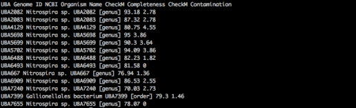
Results: Cld is present in 11 genomes in the genus Nitrospira (expected) and 1 genome in the order Gallionellales (unexpected!).  The interesting genome, UBA7399 Gallionellales, is 79.3% complete and 1.46% contaminated, which is not great but not bad.

Align with reference proteins and build a phylogenetic tree

Before proceeding with your analyses, I highly suggest you create an alignment and phylogenetic tree to confirm the new proteins contain any key amino acids and have the correct phylogenetic placement. I open and view alignments and trees in graphical user interfaces, specifically AliView and MEGA.

# Align reference proteins with hits and outgroup proteins
# Note: Alignment is computationally intensive for longer/more sequences
ALL_PROTEINS=./OUTPUT/all-${PROTEIN}
cat $REFERENCE $OUTGROUP $HITS > $ALL_PROTEINS.faa
muscle -in $ALL_PROTEINS.faa -out $ALL_PROTEINS.aln

# Create tree (default settings for simplicity)
FastTree $ALL_PROTEINS.aln > $ALL_PROTEINS.tre

# Open and view the align with GUI software such as AliView 
# Open and view the tree with GUI software such as MEGA
# Edit PDF in Adobe Illustrator or InkScape if you're fancy

Results: The alignment and tree are as expected. Cld from Nitrospira spp. group with Cld from previously sequenced Nitrospira. The Cld UBA7399_00885 from genome UBA7399 Gallionellales has lower sequence identity to other proteins but groups with Cld from characterized perchlorate- and chlorate-reducing bacteria, specifically those in the Betaproteobacteria (data not shown). I am assuming that Gallionellales strain is a (per)chlorate-reducing bacterium and will save its genome for later comparative studies.

Conclusions and Next Steps

With the above workflow, you have obtained:

• An HMM model for searching proteomes
• A list of protein hits above a significance threshold
• Protein sequences for hits
• Information on which UBA genomes contained hits
• An alignment of hits with reference protein sequences
• A phylogenetic tree of hits with reference protein sequences

Where you go from here depends on your scientific question. In most cases, you will save the specific subset of UBA genomes you’re interested in so that you can inspect those genomes further. You may want to confirm that genes on the same contig on your hit match the assigned phylogeny of the UBA genome.

For my analysis, it’s rather interesting that UBA7399 Gallionellales contains cld. A quick BLAST search of its ribosomal protein S3 sequence, found by a simple word search, supports its assignment in the Gallionellales, making it the first such taxon to contain cld.  In a first, it contains no other known genes for perchlorate reduction, chlorate reduction, or nitrite oxidation, and the genes in close proximity to cld are not informative. However, my own research has encountered the widely known fact that horizontally transferred genes, such as those for perchlorate and chlorate reduction, assemble poorly from metagenomes, and the genome is only ~80% complete. It’s helpful to remember that the maxim “absence of evidence is not evidence of absence” is especially true in genome-resolved metagenomics.

Other Examples

I don’t intend to use any of the following data but want to show a couple of additional examples.

Dissimilatory sulfite reductase alpha subunit (DsrA)

DsrA is half of the DsrAB dimer and essential for dissimilatory sulfate reduction, a widespread and important process. When using my dsrA.hmm and an E-value < 1e-100, the 7,280- genome bacterial UBA dataset contains 60 metagenome-assembled genomes with dissimilatory sulfite reductase, which are listed below. In comparison, the Anantharaman et. al 2018 paper identified dsrA in 123 metagenome-assembled genomes from over 4,000 genomes, including several phyla never before associated with dissimilatory sulfate reduction. One of those phyla, the Acidobacteria, is again represented here!

NCBI Organism Name, CheckM Completeness, CheckM Contamination

Acidobacteria bacterium UBA6911 [phylum] 86.38 5.13
Anaerolineales bacterium UBA5796 [order] 95.91 2
Deltaproteobacteria bacterium UBA3076 [class] 94.03 1.98
Deltaproteobacteria bacterium UBA5754 [class] 80.36 0.6
Desulfarculales bacterium UBA4804 [order] 91.29 1.29
Desulfatitalea sp. UBA4791 [genus] 74.09 3.55
Desulfobacter sp. UBA2225 [genus] 95.86 1.29
Desulfobacteraceae bacterium UBA2174 [family] 96.13 1.94
Desulfobacteraceae bacterium UBA2771 [family] 89.19 1.29
Desulfobacteraceae bacterium UBA4064 [family] 97.42 0.32
Desulfobacteraceae bacterium UBA4769 [family] 95.48 1.94
Desulfobacteraceae bacterium UBA5605 [family] 91.61 0.32
Desulfobacteraceae bacterium UBA5616 [family] 93.55 2.96
Desulfobacteraceae bacterium UBA5623 [family] 83.26 2.47
Desulfobacteraceae bacterium UBA5746 [family] 94.84 2.37
Desulfobacteraceae bacterium UBA5852 [family] 91.54 6.16
Desulfobulbaceae bacterium UBA2213 [family] 58.77 1.75
Desulfobulbaceae bacterium UBA2262 [family] 89.16 4.96
Desulfobulbaceae bacterium UBA2270 [family] 90.75 6.85
Desulfobulbaceae bacterium UBA2273 [family] 99.34 0.2
Desulfobulbaceae bacterium UBA2276 [family] 66.62 1.49
Desulfobulbaceae bacterium UBA4056 [family] 71.93 1.75
Desulfobulbaceae bacterium UBA5121 [family] 95.45 0.6
Desulfobulbaceae bacterium UBA5123 [family] 75.45 1.66
Desulfobulbaceae bacterium UBA5173 [family] 70.97 1.79
Desulfobulbaceae bacterium UBA5611 [family] 70.18 0.88
Desulfobulbaceae bacterium UBA5628 [family] 53.42 0
Desulfobulbaceae bacterium UBA5750 [family] 75.44 1.75
Desulfobulbaceae bacterium UBA6913 [family] 94.95 1.79
Desulfomicrobium sp. UBA5193 [genus] 98.15 0
Desulfonatronaceae bacterium UBA663 [family] 90.26 0.89
Desulfovibrio magneticus [species] 93.15 3.04
Desulfovibrio sp. UBA1335 [genus] 73.67 0.89
Desulfovibrio sp. UBA2564 [genus] 84.95 0.26
Desulfovibrio sp. UBA4079 [genus] 90.88 0.59
Desulfovibrio sp. UBA6079 [genus] 100 0
Desulfovibrio sp. UBA728 [genus] 77.15 0.3
Desulfovibrio sp. UBA7315 [genus] 54.44 0.3
Desulfovibrionaceae bacterium UBA1377 [family] 98.08 0.59
Desulfovibrionaceae bacterium UBA3823 [family] 82.63 1.18
Desulfovibrionaceae bacterium UBA3867 [family] 76.06 0.26
Desulfovibrionaceae bacterium UBA5546 [family] 100 0
Desulfovibrionaceae bacterium UBA5821 [family] 85.94 2.96
Desulfovibrionaceae bacterium UBA5842 [family] 96.91 0
Desulfovibrionaceae bacterium UBA6814 [family] 83.36 3.25
Desulfovibrionaceae bacterium UBA930 [family] 81.38 2.66
Firmicutes bacterium UBA3569 [phylum] 76.89 0.77
Firmicutes bacterium UBA3572 [phylum] 98.41 0
Firmicutes bacterium UBA3576 [phylum] 79.24 0
Firmicutes bacterium UBA911 [phylum] 81.21 0.64
Moorella sp. UBA4076 [genus] 75.09 1.57
Nitrospiraceae bacterium UBA2194 [family] 95.45 2.73
Syntrophaceae bacterium UBA2280 [family] 96.77 5.48
Syntrophaceae bacterium UBA4059 [family] 92.58 2.58
Syntrophaceae bacterium UBA5619 [family] 80.27 4.03
Syntrophaceae bacterium UBA5828 [family] 84.48 3.23
Syntrophaceae bacterium UBA6112 [family] 83.53 3.23
Thermodesulfobacteriaceae bacterium UBA6232 [family] 90.74 2.16

Cytoplasmic Nar nitrate reductase (cNarG) and periplasmic nitrate reductase (NapA)

Denitrification and dissimilatory nitrate reduction to ammonia are important processes in agriculture and just about any other system with active nitrogen redox cycling, and Nar and Nap are the primary nitrate reductases involved. A very quick glance (shows that many genomes in the UBA dataset have cnarG (776 genomes; E-value < 1e-200) or napA (361 genomes; E-value < 1e-200). This is a case where there are too many proteins to create a phylogenetic tree easily, so here’s a barplot:

Polyketide synthases

Polyketide synthases are important secondary metabolite biosynthesis proteins and tend to make the news when new ones are discovered. I very lazily copied the seed for pfam 14765, the polyketide synthase dehydratases, chose an arbitrary E-value threshold (< 1e-50) without verifying whether it was too low or too high, and aligned full-length PKS “hits” with the partial length pfam 14765 seed sequences, so this is not a correct analysis.  But there are clearly polyketide synthases in the UBA dataset. Have fun!

Addenda: Limitations and Alternatives

EDIT: A proposal for the ethical use of this dataset

Upon reflection, I felt the need to add this section. Many researchers invested significant resources into sequencing metagenomes. I believe that while the UBA dataset has done a public service by assembling so many metagenomic reads that would never be assembled and binned, many metagenomic assemblies must have been published before researchers were ready to release them. This tutorial could accelerate the “scooping.” In your use of this dataset, please avoid using information from metagenomes that have not been published and state an intent to use similar data. For example, if you are studying nitrogenase genes and find a dataset rich with interesting nitrogenase genes, I argue that it is unethical to include those genes in your analysis if the metagenome’s stated purpose is to study nitrogenases – unless they’ve already published the work. Maybe you disagree. But would you want someone to steal your dissertation research? Obviously not.

How to find this information (using the Cld example):

1. Find the SRA accession in the field “SRA Bin ID” (e.g. SRX332015);
2. Navigate to the webpage of the SRA found at “https://www.ncbi.nlm.nih.gov/sra/SRA#########[accn]” (e.g. SRX332015[accn])
3. Select “BioProject” from the “Related Information” panel on the right (e.g. PRJNA214105);
4. Inspect the description of the BioProject (e.g. no information makes me concerned about using Cld sequences or a single genome from this sample).
5. Record which BioProjects you can use and the SRAs belonging to them.

Script

I have created a bash script, available on github, to run all of the above code after the download and  preparation of the UBA bacterial dataset. Edit the path to your HMMs and reference proteins in the script, then run using the following command:

 sh uba-hmmer-pipeline.sh <protein> <E-value threshold>

Low memory

If you do not have a computer cluster or hard drive with enough memory to handle the 267 Gb total created by this workflow, you should consider downloading and processing the dataset in parts.

Try this nested for-loop, which should create no more than ~65 Gb at any one time and result in a ~7 Gb FASTA file of proteins. I did not test this, and you will probably need to change the directory “bacteria” to the directory created by unpacking the download in parts. You may find it easier to download one at a time manually.

# For parts 00 through 05
for NUM in 00 01 02 03 04 05;
do

# Download annotations for all UBA bacterial genomes
wget https://data.ace.uq.edu.au/public/misc_downloads/uba_genomes/uba_bac_prokka.part-$NUM . ;

# Unpack the tarball and promptly remove it to save space
cat uba_bac_prokka.part-$NUM | tar xz
rm uba_bac_prokka.part-$NUM

# Collect proteins
for GENOME in `ls bacteria/`; 
do 
sed "s|.*_|>${GENOME}_|" bacteria/${GENOME}/${GENOME}.faa | cat >> uba-bac-proteins.faa; 
done

rm -r bacteria/

done

Searching for nucleotides or other information in genomes

The above tutorial covers searching for proteins, but you can easily search this dataset for genes in nucleotide sequences, for example, using BLASTN directed at *ffn files. The available genome annotations are standard output from prokka:

• .gff This is the master annotation in GFF3 format, containing both sequences and annotations. It can be viewed directly in Artemis or IGV.
• .gbk This is a standard Genbank file derived from the master .gff. If the input to prokka was a multi-FASTA, then this will be a multi-Genbank, with one record for each sequence.
• .fna Nucleotide FASTA file of the input contig sequences.
• .faa Protein FASTA file of the translated CDS sequences.
• .ffn Nucleotide FASTA file of all the prediction transcripts (CDS, rRNA, tRNA, tmRNA, misc_RNA)
• .sqn An ASN1 format “Sequin” file for submission to Genbank. It needs to be edited to set the correct taxonomy, authors, related publication etc.
• .fsa Nucleotide FASTA file of the input contig sequences, used by “tbl2asn” to create the .sqn file. It is mostly the same as the .fna file, but with extra Sequin tags in the sequence description lines.
• .tbl Feature Table file, used by “tbl2asn” to create the .sqn file.
• .err Unacceptable annotations – the NCBI discrepancy report.
• .log Contains all the output that Prokka produced during its run. This is a record of what settings you used, even if the –quiet option was enabled.
• .txt Statistics relating to the annotated features found.
• .tsv Tab-separated file of all features: locus_tag,ftype,gene,EC_number,product

Incomplete genomes

Most of the metagenome-assembled genomes from the UBA dataset are less than 90% complete, which means they seem to be less complete than most closed genomes. As noted above, this can lead to the absence of important genes that can inform your analysis. Also, here’s how the assembly of UBA genomes is described in the methods:

Each of the 1,550 metagenomes were processed independently, with all SRA Runs within an SRA Experiment (that is, sequences from a single biological sample) being co-assembled using the CLC de novo assembler v.4.4.1 (CLCBio)

That is, single samples were used for assembly and binning. It’s known that assembling reads from multiple samples can improve the assembly of rare genomes and deteriorate the assembly of common genomes. It’s also known that differential coverage information – reads mapped from multiple samples with varying strain abundances – improves binning. In summary, it’s likely that many bins could be improved through more careful binning of a few samples. You can try to assemble and bin these genomes yourself using Anvi’o.

Genomes without protein annotations

You can obtain structural annotations for any genome sequence quickly using prodigal, which is the backbone of prokka.

prodigal -i genome.fna -a proteins.faa -d genes.ffn

Other datasets

Obviously, you might be more interested in other sets of genomes. I provide some options in another tutorial here.

Citations

UBA genomes:

• Parks DH, Rinke C, Chuvochina M, Chaumeil P-A, Woodcroft BJ, Evans PN, et al. (2017). Recovery of nearly 8,000 metagenome-assembled genomes substantially expands the tree of life. Nat Microbiol 2: 1533–1542.

Other genome-resolved metagenomics papers demonstrating some useful practices. Disclosure: I work closely with the Banfield lab, and one of these papers is my own.

• Anantharaman K, Hausmann B, Jungbluth SP, Kantor RS, Lavy A, Warren LA, et al. (2018). Expanded diversity of microbial groups that shape the dissimilatory sulfur cycle. ISME J. e-pub ahead of print, doi: 10.1038/s41396-018-0078-0.
• Anantharaman K, Brown CT, Hug LA, Sharon I, Castelle CJ, Probst AJ, et al. (2016). Thousands of microbial genomes shed light on interconnected biogeochemical processes in an aquifer system. Nat Commun 7: 13219.
• Barnum TP, Figueroa IA, Carlström CI, Lucas LN, Engelbrektson AL, Coates JD. (2018). Genome-resolved metagenomics identifies genetic mobility, metabolic interactions, and unexpected diversity in perchlorate-reducing communities. ISME J 12: 1568–1581.
• Crits-Christoph A, Diamond S, Butterfield CN, Thomas BC, Banfield JF. (2018). Novel soil bacteria possess diverse genes for secondary metabolite biosynthesis. Nature 558: 440–444.