
Note: This is a tutorial to help other microbiologists learn a research method from a recent publication (EDIT: open-access PDF). This method can be applied to de novo genome and metagenome assemblies from short read sequencing data (e.g. Illumina) but is not relevant for assemblies using long read sequencing data (e.g. PacBio).
Code In Brief
As the below article details, I recommend that all genome-resolved metagenomic studies use Bandage to inspect assembly graphs, at a minimum, to check for (1) abundant genomes that have been critically mis-assembled and (2) genes crucial to your study that may not have been binned.
To create a subgraph for #1 and render an image:
Bandage reduce k99.fastg graph.gfa --scope depthrange --mindepth 500.0 --maxdepth 1000000 --distance 3
Bandage image graph.gfa graph.png --nodewidth 50 --depwidth 1
To create a subgraph for #2:
Bandage reduce k99.fastg reduced.gfa --query keygene.fasta --scope aroundblast --evfilter 1e-20 --distance 5
The path to Bandage commands on a Mac is: /Applications/Bandage.app/Contents/MacOS/Bandage
Outline
- Introduction
- Preparing the Assembly Graph
- Assessing and Improving Genome Binning
- Recovering Specific Sequences
- Future Directions and Lessons
- Addendum: Alternatives
I. Introduction
The algorithms used to assemble genomes and metagenomes from short sequencing reads have a fundamental problem. When a genome contains two or more identical sequences, the algorithm will combine them into one consensus sequence instead of a producing unique contigs for every sequence. To show why this is an issue, consider what would happen if an algorithm, set to use 5-letter substrings, assembled the following sentence:
“Everything is everywhere but the environment selects.” (depth=1x)
Because the substring “every” appears twice, the assembly algorithm combines them as a consensus sequence. Consequently, the algorithm cannot determine the correct order of the sequences. The result is a fragmented sequences, with the repetitive sequence as the point of fracture:
“Every” (2x)
“thing is” (1x)
“where but the environment selects.” (1x)
Clearly, much of the meaning is lost. (Though some would argue the meaning of the sentence has been improved).
Although genome assemblies involve nucleotides and longer substrings than the example above, they suffer from the same flaw: a repetitive sequences will fragment one long sequence into several smaller sequences. Metagenome assemblies are extra complicated because related microbes can have mostly, but not entirely, identical genomes, creating mis-assemblies caused by what I will refer to as “strain variation.” The combination of repetitive sequences, caused by duplication and horizontal transfer, and strain variation, caused by conserved sequences amid varying sequences, presents two major issues for metagenome assembly. First, the mis-assembly of specific sequences which limits recovery of important genes, like the highly conserved gene for 16S ribosomal RNA. Second, the fragmentation of genomes into many smaller contigs, which limits genome recovery using assembly and binning. These issues are related – what is genome fragmentation but the mis-assembly of many sequences? – but pose different problems for different analyses.
Assembly graphs, also known as contig graphs and de Bruijn graphs, can help remedy the problems posed by mis-assembly. Analyzing assembly graphs with a tool such as Bandage (a Bioinformatics Application for Navigating De novo Assembly Graphs Easily) [1] provides crucial context for correcting mis-assemblies in a simpler format than read-mapping, a complementary tool. As shown in the below video, with assembly graphs you can quickly intuit the quality of the assembled genome and methodically diagnose mis-assemblies, such multiple copies of the 16S rRNA gene interfering with one another’s assemblies.
In a recent publication [2], I used assembly graphs of a metagenome assembly to fix mis-assembled sequences and assign them to “bins,” the collections of contigs constituting a metagenome-assembled genome. Because these mis-assembled sequences were the primary subject of the research, the publication of the study absolutely depended on assembly graphs for the recovery of the sequences. Your needs may not be as dire, but assembly graphs could still prove useful. Below, I use the published data to describe how to recover specific sequences and assess genome binning quality, which was not detailed in the publication but is likely to be helpful in almost any metagenome study.
First, a little background on the research. I study a metabolism called perchlorate reduction, in which bacteria use a modified electron transport chain to respire perchlorate (ClO4-). (How and why some bacteria get their energy from perchlorate, which rains down from the atmosphere in only the tiniest amounts, is fascinating, understudied, and not at all relevant here). Only isolated perchlorate-reducing bacteria have been studied, so not much was known about the diversity of uncultivated perchlorate reducers and how they might interact with other organisms. By performing metagenome sequencing on communities fed perchlorate, I hoped to find out which microbes reduced perchlorate and which did something else. The only problem? The genes for perchlorate reduction, perchlorate reducatase (pcr) and chlorite dismutase (cld), are horizontally transferred, so different organisms possessed highly similar sequences of the same genes. As you can now predict, most copies of pcr and cld were divided between short contigs and impossible to accurately bin – a far too common problem in metagenomic datasets.
II. Preparing the Assembly Graph
Limitations and Strategies
Before you attempt to use assembly graphs in metagenomics, please note that currently, it is very hard to work with larger metagenomic datasets. Ryan Wick, the developer of Bandage, provides some helpful tips for dealing with large metagenomic datasets that you should read fully. I have been able to apply this technique to a metagenome of about 80 recovered genomes and 1,000 Mbp total sequence (2.6 Gb file, unpublished results), but it was exceptionally slow and frustrating. I predict that for any metagenome with >40 recovered genomes, reducing the dataset’s complexity will greatly improve the speed and utility of your assembly graphs analysis.
One strategy to reduce the complexity of the metagenomic dataset is to assemble each sample independently. Most metagenome assemblies combine all reads to increase coverage, but assembling samples individually provides its own advantages. Specifically, it both reduces the total size of each assembly (increasing Bandage’s speed) and, importantly, decreases the likelihood that a closely related genome/sequence is present (lowering the chance of mis-assembly). The cost is in coverage (fewer genomes recovered) and, in some cases, time and memory required to analyze samples one-by-one. A compromise would be to assemble similar samples together.
A complementary strategy is to subsample reads prior to assembly. Essentially, selecting a subset of reads filters out low-abundance genomes that create mis-assemblies from strain variation. The downside is that perfectly fine, less-abundant genomes are also removed. seqtk has a convenient subsampling tool.
# Subsample 1% of reads to a new file
SUB=0.01
RANDOM_STRING=100
seqtk sample -s $RANDOM_STRING f.fastq $SUB > ${SUB}_f.fastq
seqtk sample -s $RANDOM_STRING r.fastq $SUB > ${SUB}_r.fastq
Note: if you do use either of these strategies to assist with genome binning, you can use dRep to de-replicate the genomes recovered from multiple assemblies. (dRep was developed by my colleague, Matthew Olm).
A final simple strategy to reduce the complexity of the graph is to run the Bandage “reduce” command from a command line (not available within the GUI). This command subsamples the assembly graph according to specific parameters, including contigs/nodes within a certain range of read depth (caution: within-genome variation can be rather large) or within a certain distance from a BLAST hit or node of interest (caution: at high distances, e.g. >20, this can capture multiple genomes). Using a reduced graph will quickly and painlessly improve Bandage’s performance but will not correct any inherent issues in the assembly arising, for example, from strain variation.
Try a total assembly yourself, then see if you need to take extra measures to reduce the datasets’ complexity.
Creating the Assembly Graph
Bandage supports assembly graphs produced by several different assemblers (see: supported formats). I used MEGAHIT (FASTG format), which requires an additional command after assembly to generate the assembly graph. For example:
# Trim reads prior with Sickle
sickle pe -f f.fastq -r r.fastq -t sanger -o f_trimmed.fastq -p r_trimmed.fastq -s singles_trimmed.fastq q=20

# Assembly
megahit -1 f_trimmed.fastq -2 r_trimmed.fastq -o output
# MEGAHIT also has presets for different types of metagenomic datasets
# After assembly
cd output/intermediate_contigs
megahit_toolkit contig2fastg 99 k99.contigs.fa > k99.fastg
open k99.fastg
Bandage developers have supplied a sample genome assembly to inspect. If you would like to try out using assembly graph on a metagenomic dataset, you can download, trim, and assemble reads from a simple, 4-genome community observed in my study.
Scaffolding vs. Assembly Graphs
Scaffolding is a method to extend and combine contigs that produces more-complete metagenome-assembled genomes. Assembly graphs, however, are composed of contigs, not scaffolds. If you would like to use assembly graphs from a metagenomic dataset that has been scaffolded, you must parse your scaffolding output to find the contigs within each scaffold within each bin. How to find and parse this information will vary by scaffolding method. (For the scaffolding algorithm SSPACE, the relevant information is in the files “*.final.evidence” and “*.formattedcontigs_min0.fasta”). If you’re bold, you may skip scaffolding, which has worked for me on very enriched communities with fewer genomes and less strain variation.
III. Assessing and Improving Genome Binning

- Include sequences too short for binning algorithms (<2000-2500 bp).
- Include sequences of too aberrant coverage for binning algorithms (e.g. rRNA genes)
- Identify misbinned sequences within a contiguous assembly.
- Identify strain variation in abundant genomes, which can inform the subsampling of samples or reads.
- In rare cases, create complete, finished genomes.
I’ll explain each of these uses below. First, some basics. You can highlight a specific bin by selecting its contigs/nodes:
# Create list
BIN=bin001
grep '>' ${BIN}.fasta > ${BIN}.headers.txt # Select contigs
sed 's/>k99_//' ${BIN}.headers.txt > ${BIN}.nodes.txt # Remove prefix
sed -i 's/$/,/' ${BIN}.nodes.txt # Add comma to end of line
# Copy and paste list into Bandage to color/label
More comprehensively, you can color and label many bins at once using a CSV file. Here are the specifications provided to me by Ryan Wick:
The feature currently works as follows: if a column in your loaded CSV file has a header of “color” or “colour” (case insensitive), then the values in that column are treated as colours. The values can specify the exact colour, either as 6-digit hex (e.g. #FFB6C1), an 8-digit hex with transparency (e.g. #7FD2B48C) or a standard colour name (e.g. skyblue). If the value does not fit any of those, then it is considered a category and assigned a colour automatically. All nodes with the same category will obviously get the same colour. These colours are assigned as the nodes’ custom colours, not as a new colour category.
For example:
Name,color,bin,label
17986,2F6D80,Bin001,The10000thClostridia
55081,67CAD5,Bin002,CPR-HostUnknown:(
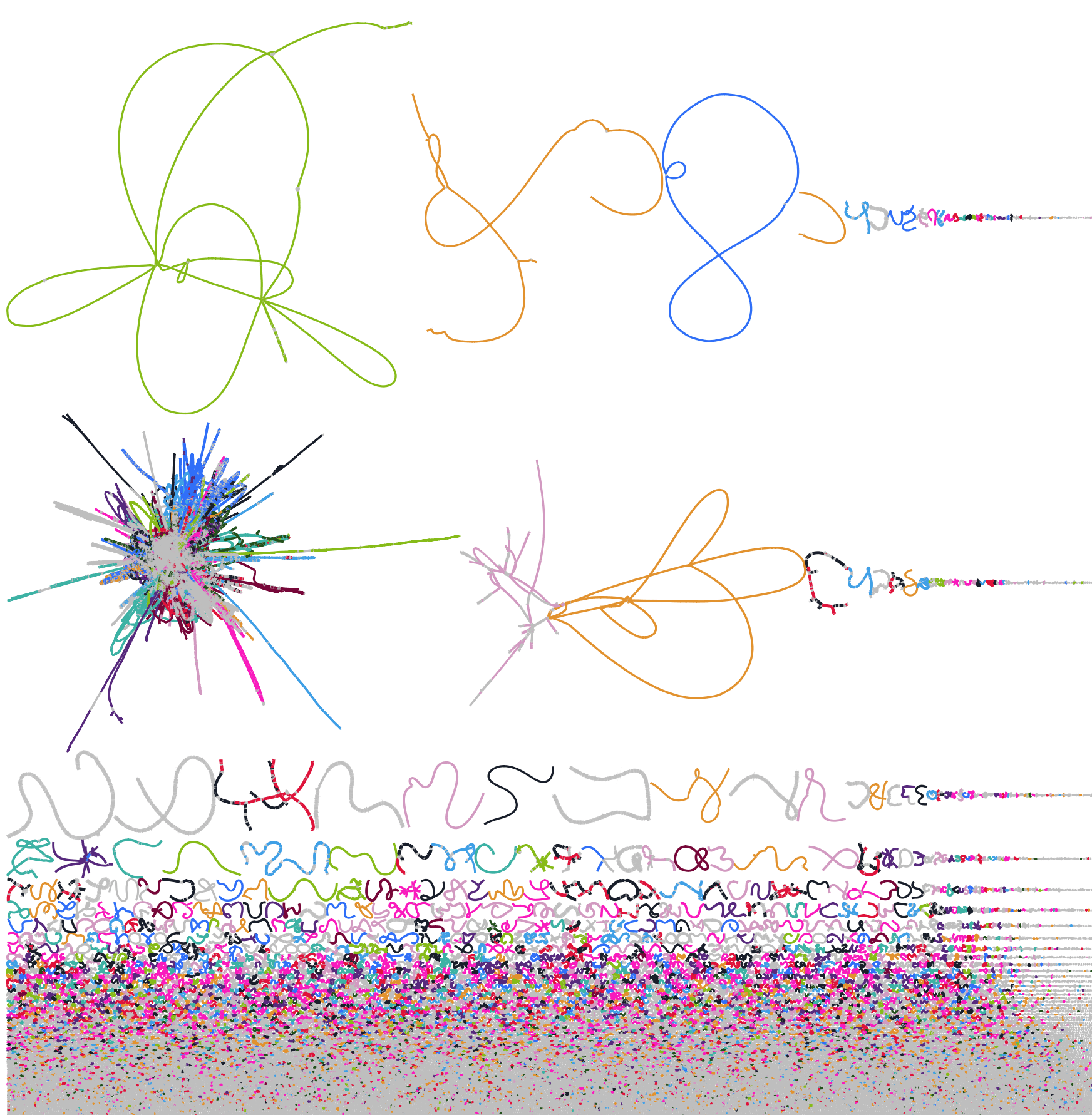
For Anvi’o users, I have written a (novice) Python script that generates the CSV file for labeling bins. (EDIT: Antti Karkman at the University of Gothenburg has provided an edited script that for contigs that have been renamed and filtered using ‘anvi-script-reformat-fasta’). The script cycles through a limited set of 12 colorblind-safe colors, since people can only discriminate between 6-8 colors at once anyway. (I suggest that you focus in on closely related organisms, since those are more likely to be spatially adjacent in assembly graphs). The result is enlightening:


You can immediately notice which bins are near-complete with long, interrupted contigs and which bins have related genomes that interfered with assembly. If you did a good job binning, this image will be rather pleasing. It’s also a helpful educational display.
Even after rigorous binning, you can notice binning errors in the published dataset*; some sequences are indicated as unbinned (gray), probably because I excluded low quality bins from the analysis, and some bins have minor errors. Most researchers accept that any metagenome-assembled genome may have some contamination and that you cannot fix every error (one memorable quote: “you will get garbage from metagenomic assemblies”), but for those who seek be as rigorous as possible, as when identifying a new metabolism or a new phylum, this method will support your case. Below are some examples of common uses for assembly graphs in binning.
Include sequences too short for binning algorithms (<2000-2500 bp) & sequences of too aberrant coverage for binning algorithms (e.g. rRNA genes)
The short and/or abundant sequences could have been binned with the surrounding bin.
To include all nodes that are contiguous with a genome bin, you can create a reduced graph extended from the binned contigs. Be aware that some bins can be connected to dozens of others, so you should be selective.
# Remove new line characters from list of nodes
tr -d '\n' < bin001.nodes.txt > bin001.inline.nodes.txt

# Select all contiguous nodes to bin001
Bandage reduce k99.fastg bin001.gfa --scope aroundnodes --distance 50 --nodes `cat bin001.inline.nodes.txt`
# Load the Bandage GUI, load the CSV, and reinspect the bins
Identify misbinned sequences within a contiguous assembly.
The contigs in the red bin clearly belong in the purple bin. These errors become more common when strain variation is present, as indicated by the many breaks between contigs.

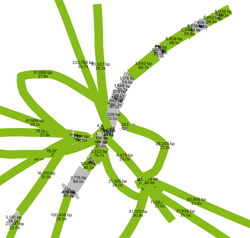
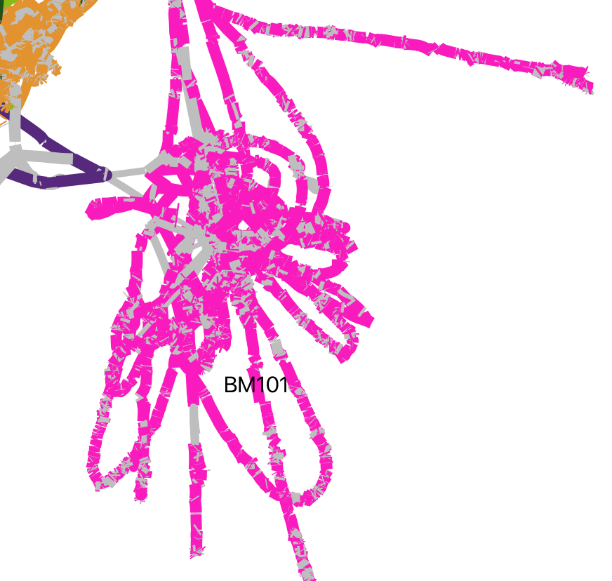
Identify strain variation in abundant genomes, which can inform the subsampling of samples or reads.
Genome BM101 was not happy to be assembled, likely due to the presence of multiple strains in the enrichment.
An important aside: While CheckM determined this bin to be 98% complete with 3% contamination, as judged by conserved single copy genes, we can clearly see that many accessory genes will be interrupted in or absent from the published metagenome-assembled genome. The true completeness of the genome was overestimated because the conserved sequences of the core genome were better assembled than variable genes. Additionally, binning tends to remove genes that have been adaptively gained or lost between samples. Together, this means that the estimated completeness of metagenome-assembled genomes is greater than that of the true genome.
Unfortunately, because strain variation is essentially the recreation of slightly diverged sequences, simply using Bandage to select all the contigs/nodes of a genome affected by strain variation can produce a genome bin with many more nucleotides and genes than the true genome. In this case, the completeness estimates may underestimate the genome’s duplicity. If strain 1 and strain 2 have very different coverage, a subsampling approach as discussed above may help disentangle one from the other. A fancier-though-not-always-better approach is to (1) select all of the contigs, (2) select all reads that mapped to those contigs from your BAM file, (3) subsample that subset of reads, and (4) assemble each subsampled subset. Decide before you start how desperate you are for a clean genome.
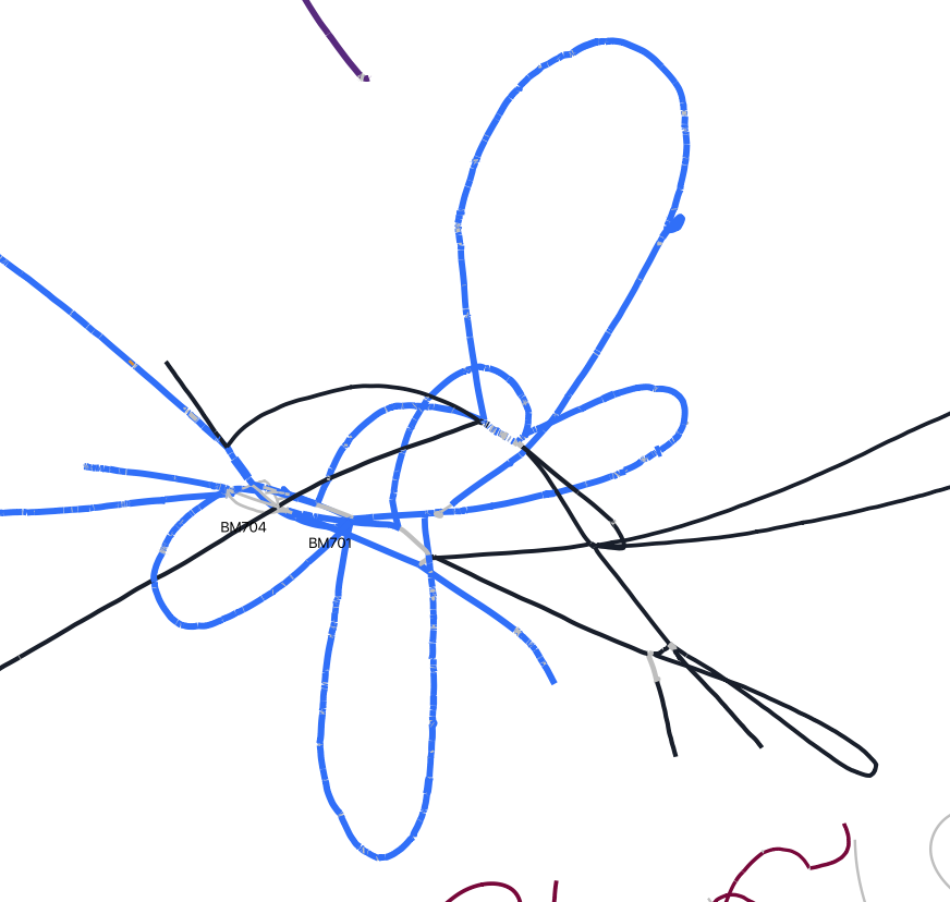
Strain variation can also be much more benign, as in the case of these genomes from the genus Denitrovibrio which are much more well-assembled and binned.
In my experience, strain variation is more likely to affect more-abundant genomes. There may be a biological reason for this, but it could simply be that less-abundant genomes do not have sufficient coverage of the minority strain to create an issue. For example, if two strains are in a ratio of 10:1 and a genome requires 4x coverage to assemble, assembly problems that are significant at 1000x coverage (1000x:100x) would be insignificant at 10x coverage (10x:1x) where the minority strain would not assemble by itself alone (1x < 4x).
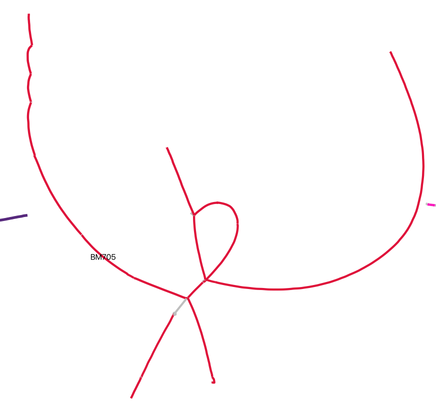
In rare cases, create complete, finished genomes.
Manual assembly may have been to reduce this small CPR bacteria genome from 81 nodes to 8 nodes, which could then be scaffolded with manual read mapping.
The subsampling strategies discussed above are particularly useful for recovering complete genomes.
The Importance of Assessing and Improving Genome Binning
After completing a round of automated binning, you can assess your bins to an assembly graph to diagnose problems with binning such as strain variation and inaccurate binning. For example, in one metagenome assembly, strain variation so bad that the most abundant genome was undetected in binning because it was entirely fragmented into ~1000-bp contigs. After recovering a genome by assembling samples individually, the strain was found to have a key functional role! Highlighting bins in an assembly graph is one way to identify this example.

Let this be a cautionary tale that you should at a minimum check a reduced assembly graph of the most abundant contigs for short, unbinned sequences.
# Select nodes >500x coverage and three connected nodes to maintain links
Bandage reduce k99.fastg graph.gfa --scope depthrange --mindepth 500.0 --maxdepth 1000000 --distance 3
Assembly graphs can improve most genome bins by capturing contigs too short or too aberrant in coverage. While this can consume as much time as you let it, you may be able to be more efficient and reproducible by automating processes. Alternatively, you can consider this a curation step for a genome(s) of special interest.
Note: For my publication, I relied exclusively on standard approaches for binning (i.e. Anvi’o), as most groups do, but the errors above indicate that bin recovery could have been improved by inspecting the assembly graph. Fortunately, none of the errors change the conclusions of the paper, but I still plan to update revised genomes to NCBI.
IV. Recovering Specific Sequences
Assembly graphs have a second important use: using qualitative information to assemble sequences that an algorithm cannot. Assembly graphs enabled me to manually assembly highly conserved sequences (16S rRNA genes) and horizontally transferred sequences (pcr and cld) that were crucial to my research. The goals are to merge short contigs belonging to a fragmented sequence and to link them to longer contigs that belong to genome bins. From the paper:
“Bandage . . . . was used to visualize contigs, identify BLAST hits to specific gene sequences, manually merge contigs, and relate merged contigs to a genome bin. Criteria for merging contigs were that contigs (1) shared a similar abundance and (2) lay in the same contiguous path. Merged contigs were binned when contiguity with multiple contigs from the same genome bin was certain. This strategy was also used to recover some 16S rRNA genes.”
This is particularly useful for unbinned contigs that, as you could notice in the above section, can be clearly linked to a specific genome.
Identifying and Visualizing Genes of Interest with BLAST
The first step is to identify the contigs/nodes that contain your gene of interest. You can either perform your own homology search or use the built-in BLAST annotation feature in Bandage (detailed instructions). While you may want to visualize all hits at first to understand the distribution among genomes, it is much simpler to reduce the Scope to “Around BLAST hits” or “Around [selected] nodes” and only show a short Distance of nodes. The key benefit? In a FASTA file all of these contigs appear are separate, yet in an assembly graph their spatial relationship is maintained.
Manually Merge Contigs
In Preferences, adjust Depth and Node Width to accentuate coverage differences between nodes. This helps distinguish sequences from different organisms. To merge nodes, use Output > “Specific exact path for copy/save” to input selected node sequences. (Tip: Have a list of nodes, enter one at a time, and toggle +/- until Bandage confirms the path is possible). I only merged nodes if they share the same path (“contiguous”) and had logically similar abundance. In the below example, while at much higher abundance, the 1000x contig could be a duplicated sequence flanking the selected insertion and the sequences at the bottom left.
Remember that the sequence you recover is likely a consensus sequence. Usually, an assembler will use the higher coverage nucleotides to construct the contig, but in similarly abundant reads the result could be a mixture of nucleotide identities from two or more populations. If it matters for your study, you can perform an SNV analysis.
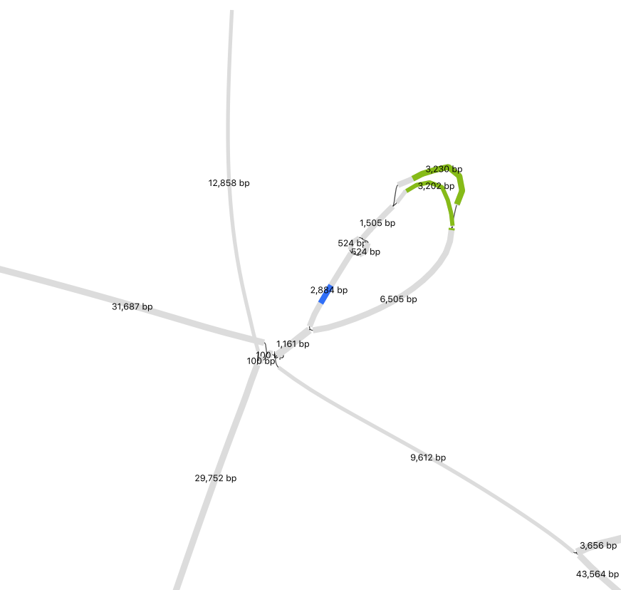
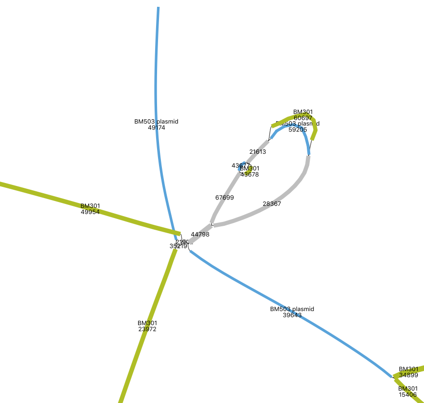
Relate Merged Contigs to a Genome Bin
Select a sequence from adjacent contigs and search for it among your bins. Often, as below with genomes “BM301” and “BM503,” the genome bin that the sequence of interest belongs to can be blindingly obvious: all contigs/nodes are contiguous and of similar abundance. (Note: reads can be recruited from similar sequences or unassembled sequences in your metagenome, distorting read depth).
From the paper:
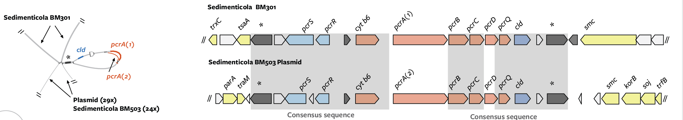
Other times, you will be less certain of the contiguity. It is best to conservative about merging and binning sequences. When necessary, you can use read mapping or even PCR to link some contigs to one another with more certainty.
Adding Sequences to Bins
Your manual assembly might include sequences that are already present in genome bins that should be removed from the genome bin before analysis. Duplicates contigs can be identified by the name of the contigs/nodes or, in the case of scaffolded sequences, by using nucmer:
nucmer --coords -prefix bin001 bin001.fasta bandage_seqs.fasta
The Importance of Recovering Specific Sequences
This method enables you to recover and bin a consensus sequence from fragmented contigs. Crucially, with this manual assembly you can determine if more than one genome contains the same sequence. I understand any aversion to using this technique for that reason, but (1) ignoring something does not mean it is not there and (2) other techniques generate duplicity anyway, as evidenced for the need for programs like dRep.
Inspecting numerous assembly graphs has convinced me that many important gene sequences fail to be properly binned. At a minimum, I advise researchers search for connections between binned sequences and important genes that might be on unbinned sequences. You can either simply eyeball the size of the results or more accurately parse the returned contigs and compare that list to binned contigs. The following Bandage command enables such a search:
# Select portion of graph within 5 nodes BLAST hits to the key gene, with E-value filter of 1e-20
Bandage reduce k99.fastg reduced.gfa --query keygene.fasta --scope aroundblast --evfilter 1e-20 --distance 5
V. Future Directions and Lessons
- Code for updating an Anvi’o database/collection using revised binning selections from Bandage.
- Automated refinement of binning by extending a bin’s graphs until it reaches another bin’s graph. This would allow binning to incorporate information from the assembler (note: this may not lead to improvements for all bins).
- Using assembly graph information to assess completeness and contamination.
- A complementary binning workflow for sequences less than <2500 bp that may constitute highly abundant genome(s) affected by strain variation. For example, all short contigs greater than 100x coverage are grouped by taxonomy. Contigs of a genome would be compared to BAM files to determine in which sample is coverage sufficiently highly and SNVs sufficiently low to enable assembly through subsampling.
- Disentangling specific consensus sequences by using SNV coverage. For example, if 4% of sites in a sequence are variable because of two unique populations at ~10x and ~2x coverage, create two sequences using the (1) ~10x coverage SNVs and shared sites and (2) ~2x coverage SNVs and shared sites. If applied to entire genomes, this could be a potent way to fix strain variation.
What have I learned from using assembly graphs? Metagenomic datasets are tremendously valuable but also complex and fraught. The contigs output by the assembler often represent the composite of multiple strains as one genome. When the diversity among reads is sufficient enough, all or part of these composite genomes assemble poorly, destroying or dividing the genome. When gene gain or loss occurs between samples, genome binning tends to remove these accessory genes, which could very well be adaptive traits relevant to the study. Until the inherent issues are resolved by new comprehensive methods, researchers will be faced with making serious subjective decisions in the form of colorful spaghettis.
VI. Addendum: Alternatives
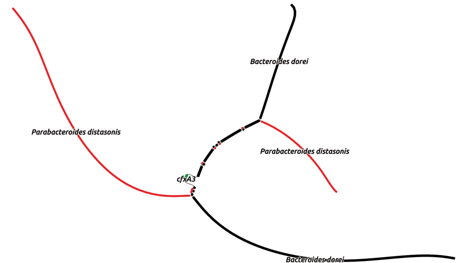
Of course, after submitting my paper and writing this blog, I found the publication describing MetaCherchant, a tool that reconstructs the genomic environment around a specific gene of interest. It is elegant, and I wish I had known about it, so I will highlight it here. MetaCherchant “builds a subgraph . . . around a target nucleotide sequence” and allows you to compare two samples to see if the genomic context of the gene has changed. MetaCherchant differs my the approach that I have described mostly in that (1) it builds a subgraph, not a graph of an entire metagenome, and (2) a specific gene of interest is used to build each graph, rather than observing multiple sequences in a single graph. Regardless, both approaches allow you to link a gene to genomes from a metagenome. Without having used the tool, I expect that MetaCherchant’s focused approach would afford some serious improvements in computational resources, time, and assembly quality if your goal is to analyze specific genes. The developers compared a total metagenome assembly from SPAdes to the localized metagenome assembly from MetaCherchant. The figure below, from their paper, shows that while the antibiotic resistance gene cfxA3 (green) to was successfully linked by both approaches (black) to the Bacteroides dorei genome, only MetaCherchant (red) linked cfxA3 to the Parabacteroides distasonis genome. That’s an important improvement in detection.
Are you instead looking for a programmatic way to improve binning? Check out Spacegraphcats, which finds groups of contigs in the assembly graph that, while hard to assemble into longer contigs, definitely belong together. Preprint here: https://www.biorxiv.org/content/10.1101/462788v1.
Ultimately, your goals and study design will inform the approach you choose.
Citing This Work
The following papers demonstrate Bandage [1] and the method and logic I used for using Bandage to recover specific sequences from metagenomic datasets [2]:
The papers for alternatives:

Thanks for sharing Tyler. This post is very helpful!
LikeLike